Andrej Karpathy blog:# The Unreasonable Effectiveness of Recurrent Neural Networks

There’s something magical about Recurrent Neural Networks (RNNs). I still remember when I trained my first recurrent network for Image Captioning. Within a few dozen minutes of training my first baby model (with rather arbitrarily-chosen hyperparameters) started to generate very nice looking descriptions of images that were on the edge of making sense. Sometimes the ratio of how simple your model is to the quality of the results you get out of it blows past your expectations, and this was one of those times. What made this result so shocking at the time was that the common wisdom was that RNNs were supposed to be difficult to train (with more experience I’ve in fact reached the opposite conclusion). Fast forward about a year: I’m training RNNs all the time and I’ve witnessed their power and robustness many times, and yet their magical outputs still find ways of amusing me. This post is about sharing some of that magic with you.
循环神经网络（RNN）有其独特的魅力。我还记得第一次训练用于图像描述生成的循环神经网络时的情景。只用了短短几十分钟，即使是随意选择的超参数，这个初步模型已经开始生成看起来非常不错的图像描述，尽管这些描述有时只是勉强合理。有时，模型的简单程度与其输出结果的质量之间的比例会远远超出预期，这次就是一个典型的例子。这次结果如此令人震惊的原因在于，当时的普遍认知是，RNN很难训练（随着经验的增加，我实际上得出了相反的结论）。时间快进大约一年：我一直在训练RNN，目睹了它们的强大和稳健，尽管如此，它们神奇的输出依然能不断带给我惊喜。这篇文章旨在与大家分享这种魔力。

We’ll train RNNs to generate text character by character and ponder the question “how is that even possible?”
我们将训练循环神经网络（RNN）逐字符地生成文本，并思考这个问题：“这到底是怎么做到的？”

By the way, together with this post I am also releasing code on Github that allows you to train character-level language models based on multi-layer LSTMs. You give it a large chunk of text and it will learn to generate text like it one character at a time. You can also use it to reproduce my experiments below. But we’re getting ahead of ourselves; What are RNNs anyway?
顺便提一下，与这篇文章一起，我还在Github上发布了代码，这些代码可以用来训练基于多层LSTM的字符级语言模型。你只需提供一大段文本，它就会逐字符地学习生成类似的文本。你还可以使用它来重现我下面的实验。但在此之前，我们还是先回到正题上来：我们先来了解一下RNN到底是什么？

Recurrent Neural Networks 递归神经网络

Sequences

Sequences. Depending on your background you might be wondering: _What makes Recurrent Networks so special_? A glaring limitation of Vanilla Neural Networks (and also Convolutional Networks) is that their API is too constrained: they accept a fixed-sized vector as input (e.g. an image) and produce a fixed-sized vector as output (e.g. probabilities of different classes). Not only that: These models perform this mapping using a fixed amount of computational steps (e.g. the number of layers in the model). The core reason that recurrent nets are more exciting is that they allow us to operate over _sequences_ of vectors: Sequences in the input, the output, or in the most general case both. A few examples may make this more concrete:
序列。根据你的背景，你可能会问：循环神经网络有什么特别之处？一个显而易见的限制是Vanilla 神经网络（以及卷积神经网络）的API过于受限：它们接受固定大小的向量作为输入（例如，一张图片），并产生固定大小的向量作为输出（例如，不同类别的概率）。不仅如此，这些模型使用固定数量的计算步骤来完成这个映射（例如，模型中的层数）。循环神经网络更令人兴奋的核心原因在于它们允许我们对向量序列进行操作：输入中的序列，输出中的序列，或者在最一般的情况下，两者都是序列。几个例子可以让这一点更加具体：

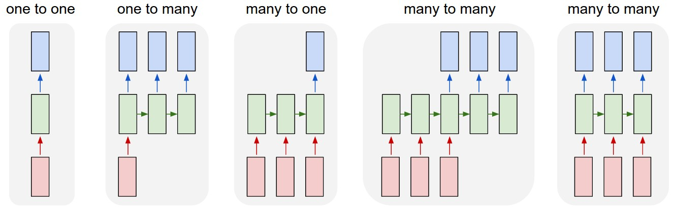
Each rectangle is a vector and arrows represent functions (e.g. matrix multiply). Input vectors are in red, output vectors are in blue and green vectors hold the RNN’s state (more on this soon). From left to right: (1) Vanilla mode of processing without RNN, from fixed-sized input to fixed-sized output (e.g. image classification). (2) Sequence output (e.g. image captioning takes an image and outputs a sentence of words). (3) Sequence input (e.g. sentiment analysis where a given sentence is classified as expressing positive or negative sentiment). (4) Sequence input and sequence output (e.g. Machine Translation: an RNN reads a sentence in English and then outputs a sentence in French). (5) Synced sequence input and output (e.g. video classification where we wish to label each frame of the video). Notice that in every case are no pre-specified constraints on the lengths sequences because the recurrent transformation (green) is fixed and can be applied as many times as we like.
每个矩形代表一个向量，箭头代表函数（例如矩阵乘法）。输入向量用红色表示，输出向量用蓝色表示，绿色向量表示RNN的状态（稍后会详细说明）。从左到右依次是：

(1) 普通模式的处理，没有使用RNN，从固定大小的输入到固定大小的输出（例如图像分类）。

(2) 序列输出（例如图像描述生成，输入一张图片，输出一个单词句子）。

(3) 序列输入（例如情感分析，将给定的句子分类为表达正面或负面情感）。

(4) 序列输入和序列输出（例如机器翻译：RNN读取一段英文句子，然后输出一段法文句子）。

(5) 同步的序列输入和输出（例如视频分类，我们希望对视频的每一帧进行标签）。

注意，在每种情况下，序列长度都没有预先指定的限制，因为循环变换（绿色）是固定的，可以根据需要应用多次。

As you might expect, the sequence regime of operation is much more powerful compared to fixed networks that are doomed from the get-go by a fixed number of computational steps, and hence also much more appealing for those of us who aspire to build more intelligent systems. Moreover, as we’ll see in a bit, RNNs combine the input vector with their state vector with a fixed (but learned) function to produce a new state vector. This can in programming terms be interpreted as running a fixed program with certain inputs and some internal variables. Viewed this way, RNNs essentially describe programs. In fact, it is known that RNNs are Turing-Complete in the sense that they can to simulate arbitrary programs (with proper weights). But similar to universal approximation theorems for neural nets you shouldn’t read too much into this. In fact, forget I said anything.
正如你所预料的那样，相较于受限于固定计算步骤的固定网络，序列操作模式要强大得多，因此对于那些希望构建更智能系统的人来说也更具吸引力。此外，正如我们稍后会看到的，RNN通过固定（但可学习）的函数将输入向量与其状态向量结合，生成一个新的状态向量。这在编程术语中可以理解为运行一个具有特定输入和一些内部变量的固定程序。从这个角度来看，RNN本质上是在描述程序。事实上，RNN被认为是图灵完备的，这意味着它们可以模拟任意程序（在适当的权重下）。但是，与神经网络的通用近似定理类似，你不应该对此过于解读。实际上，忘掉我刚才说的话吧。

If training vanilla neural nets is optimization over functions, training recurrent nets is optimization over programs.
如果说训练普通神经网络是对函数的优化，那么训练循环网络就是对程序的优化。

Sequential processing in absence of sequences. You might be thinking that having sequences as inputs or outputs could be relatively rare, but an important point to realize is that even if your inputs/outputs are fixed vectors, it is still possible to use this powerful formalism to _process_ them in a sequential manner. For instance, the figure below shows results from two very nice papers from DeepMind. On the left, an algorithm learns a recurrent network policy that steers its attention around an image; In particular, it learns to read out house numbers from left to right (Ba et al.). On the right, a recurrent network _generates_ images of digits by learning to sequentially add color to a canvas (Gregor et al.):
在没有序列的情况下进行顺序处理。您可能认为将序列作为输入或输出可能相对罕见，但需要意识到的重要一点是，即使你的输入/输出是固定向量，仍然可以使用这种强大的形式主义以顺序方式处理它们。例如，下图显示了 DeepMind 的两篇非常好的论文的结果。在左边，算法学习一个循环网络策略，将其注意力引导到图像周围;特别是，它学会了从左到右读出门牌号（Ba等人）。在右边，一个循环网络通过学习依次向画布添加颜色来生成数字图像：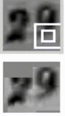

The takeaway is that even if your data is not in form of sequences, you can still formulate and train powerful models that learn to process it sequentially. You’re learning stateful programs that process your fixed-sized data.
要点是，即使你的数据不是以序列形式存在，你仍然可以设计和训练强大的模型，使其学会以顺序方式处理这些数据。你正在学习的是处理固定大小数据的有状态程序。

RNN computation

RNN computation. So how do these things work? At the core, RNNs have a deceptively simple API: They accept an input vector x and give you an output vector y. However, crucially this output vector’s contents are influenced not only by the input you just fed in, but also on the entire history of inputs you’ve fed in in the past. Written as a class, the RNN’s API consists of a single step function:
RNN 计算。那么这些东西是如何工作的呢？在核心上，RNN 有一个看似简单的 API：它们接受一个输入向量 x 并给你一个输出向量 y 。然而，至关重要的是，这个输出向量的内容不仅受到你刚刚输入的输入的影响，还受到你过去输入的整个输入历史的影响。RNN 的 API 编写为一个类，由一个 step 函数组成：

1 2	rnn = RNN() y = rnn.step(x) # x is an input vector, y is the RNN's output vector

The RNN class has some internal state that it gets to update every time step is called. In the simplest case this state consists of a single _hidden_ vector h. Here is an implementation of the step function in a Vanilla RNN:
RNN 类具有一些内部状态，每次调用时 step 都会更新。在最简单的情况下，此状态由单个隐藏向量组成 h 。以下是 Vanilla RNN 中 step 函数的实现：

class RNN:
  # ...
  def step(self, x):
    # update the hidden state
    self.h = np.tanh(np.dot(self.W_hh, self.h) + np.dot(self.W_xh, x))
    # compute the output vector
    y = np.dot(self.W_hy, self.h)
    return y

The above specifies the forward pass of a vanilla RNN. This RNN’s parameters are the three matrices W_hh, W_xh, W_hy. The hidden state self.h is initialized with the zero vector. The np.tanh function implements a non-linearity that squashes the activations to the range [-1, 1]. Notice briefly how this works: There are two terms inside of the tanh: one is based on the previous hidden state and one is based on the current input. In numpy np.dot is matrix multiplication. The two intermediates interact with addition, and then get squashed by the tanh into the new state vector. If you’re more comfortable with math notation, we can also write the hidden state update as $ℎ_𝑡=tanh⁡(𝑊_{ℎℎ}ℎ_{𝑡−1}+𝑊_{𝑥ℎ}𝑥_𝑡)$, where tanh is applied elementwise.
上述内容描述了一个基础RNN的前向传播过程。这个RNN的参数是三个矩阵W_hh、W_xh和W_hy。隐藏状态self.h初始化为零向量。np.tanh函数实现了一种非线性激活函数，将激活值压缩到[-1, 1]范围内。简要说明其工作原理：tanh内部有两个项，一个基于前一个时间步隐藏状态，另一个基于当前时间步输入。在numpy中，np.dot表示矩阵乘法。这两个中间结果通过加法相互作用，然后通过tanh函数压缩为新的状态向量。如果你对数学表示法更熟悉，我们也可以将隐藏状态的更新写成 $ℎ_𝑡=tanh⁡(𝑊_{ℎℎ}ℎ_{𝑡−1}+𝑊_{𝑥ℎ}𝑥_𝑡)$，其中tanh逐元素应用。

⚠️：numpy是Python中一个非常流行的数值计算库。np.tanh函数和np.dot函数都是numpy库中的函数。np.tanh函数用于计算元素级的双曲正切，而np.dot函数用于执行矩阵乘法。

We initialize the matrices of the RNN with random numbers and the bulk of work during training goes into finding the matrices that give rise to desirable behavior, as measured with some loss function that expresses your preference to what kinds of outputs $y$ you’d like to see in response to your input sequences $x$.
我们用随机数初始化RNN的矩阵，在训练过程中，大部分工作是找到能够产生理想行为的矩阵，这通过某种损失函数来衡量，该损失函数表达了你对输入序列$x$对应输出$y$的期望。

Going deep

Going deep. RNNs are neural networks and everything works monotonically better (if done right) if you put on your deep learning hat and start stacking models up like pancakes. For instance, we can form a 2-layer recurrent network as follows:
深入研究。RNN是神经网络的一种，如果方法得当，采用深度学习的方法并像叠煎饼一样将模型堆叠起来，一切都会单调地变得更好。例如，我们可以如下构建一个两层的循环神经网络：

1 2	y1 = rnn1.step(x) y = rnn2.step(y1)

In other words we have two separate RNNs: One RNN is receiving the input vectors and the second RNN is receiving the output of the first RNN as its input. Except neither of these RNNs know or care - it’s all just vectors coming in and going out, and some gradients flowing through each module during backpropagation.
换句话说，我们有两个独立的 RNN：一个 RNN 接收输入向量，第二个 RNN 接收第一个 RNN 的输出作为其输入。除了这些 RNN 都不知道或不关心之外——它们都只是进出的向量，以及在反向传播过程中流过每个模块的一些梯度。

Getting fancy

Getting fancy. I’d like to briefly mention that in practice most of us use a slightly different formulation than what I presented above called a _Long Short-Term Memory_ (LSTM) network. The LSTM is a particular type of recurrent network that works slightly better in practice, owing to its more powerful update equation and some appealing backpropagation dynamics. I won’t go into details, but everything I’ve said about RNNs stays exactly the same, except the mathematical form for computing the update (the line self.h = ... ) gets a little more complicated. From here on I will use the terms “RNN/LSTM” interchangeably but all experiments in this post use an LSTM.
更复杂的模型。在实践中，我们大多数人使用的公式与我上面提到的稍有不同，被称为长短期记忆网络（LSTM）。LSTM是一种特定类型的循环神经网络，实际上效果更好，因为它具有更强大的更新方程和一些更具吸引力的反向传播动态。我不会深入讨论细节，但我所说的关于RNN的一切都完全相同，除了计算更新的数学形式（即self.h = …这一行）变得稍微复杂了一些。从现在开始，我会交替使用“RNN/LSTM”这两个术语，但本文中的所有实验都使用LSTM。

Character-Level Language Models

字符级语言模型

Okay, so we have an idea about what RNNs are, why they are super exciting, and how they work. We’ll now ground this in a fun application: We’ll train RNN character-level language models. That is, we’ll give the RNN a huge chunk of text and ask it to model the probability distribution of the next character in the sequence given a sequence of previous characters. This will then allow us to generate new text one character at a time.
好的，所以我们已经对RNN是什么、为什么它们非常令人兴奋以及它们如何工作有了一定的了解。现在，我们将把这些知识应用到一个有趣的实际应用中：我们将训练RNN字符级别的语言模型。也就是说，我们会给RNN提供一大段文本，并让它根据前面字符的序列来建模下一个字符的概率分布。这样一来，我们就可以一次生成一个字符的新文本。

As a working example, suppose we only had a vocabulary of four possible letters “helo”, and wanted to train an RNN on the training sequence “hello”. This training sequence is in fact a source of 4 separate training examples: 1. The probability of “e” should be likely given the context of “h”, 2. “l” should be likely in the context of “he”, 3. “l” should also be likely given the context of “hel”, and finally 4. “o” should be likely given the context of “hell”.
作为一个实际例子，假设我们只有四个可能的字母“helo”的词汇表，并且想要在训练序列“hello”上训练一个RNN。这个训练序列实际上是四个独立的训练示例的来源：

在“h”的上下文中，“e”的概率应该很大。
在“he”的上下文中，“l”的概率应该很大。
在“hel”的上下文中，“l”的概率也应该很大。
最后，在“hell”的上下文中，“o”的概率应该很大。

Concretely, we will encode each character into a vector using 1-of-k encoding (i.e. all zero except for a single one at the index of the character in the vocabulary), and feed them into the RNN one at a time with the step function. We will then observe a sequence of 4-dimensional output vectors (one dimension per character), which we interpret as the confidence the RNN currently assigns to each character coming next in the sequence. Here’s a diagram:
具体来说，我们将使用1-of-k编码将每个字符编码成一个向量（即，除了在词汇表中字符索引处为1，其余全为0），然后用step函数将它们逐一输入RNN。随后，我们会得到一系列4维输出向量（每个字符一个维度），我们将这些输出向量解释为RNN当前对序列中下一个字符的置信度。以下是一个示意图：

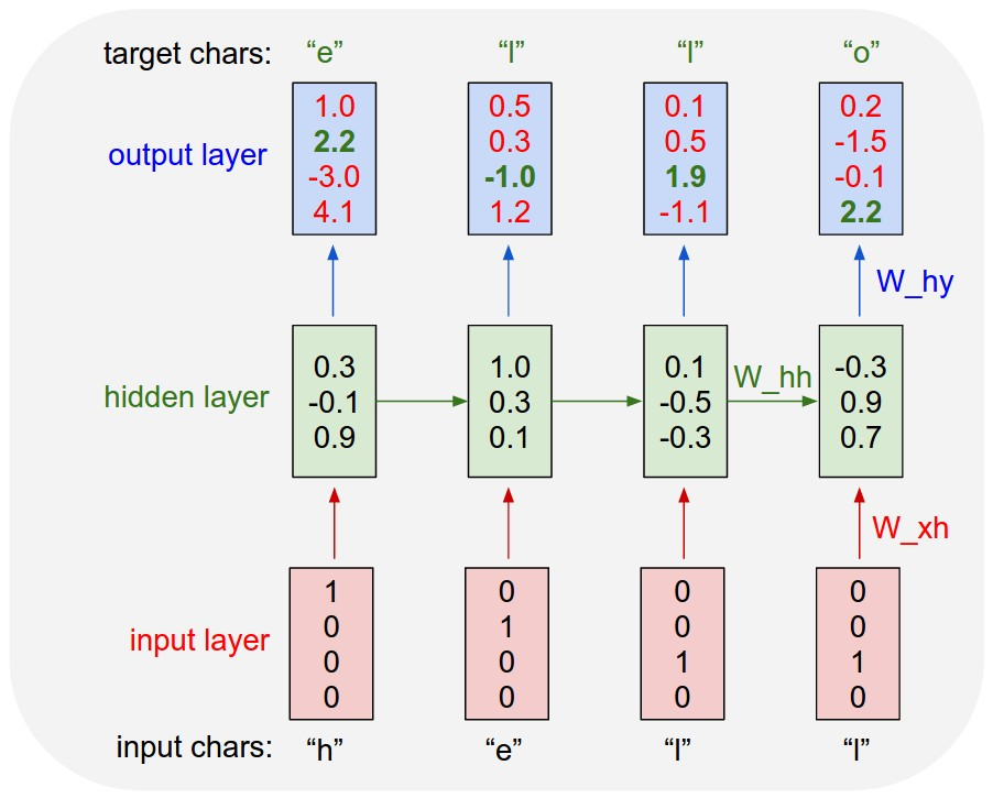
An example RNN with 4-dimensional input and output layers, and a hidden layer of 3 units (neurons). This diagram shows the activations in the forward pass when the RNN is fed the characters “hell” as input. The output layer contains confidences the RNN assigns for the next character (vocabulary is “h,e,l,o”); We want the green numbers to be high and red numbers to be low.
具有 4 维输入和输出层的示例 RNN，以及 3 个单元（神经元）的隐藏层。此图显示了将字符“hell”作为输入馈送 RNN 时前向传递中的激活。输出层包含 RNN 为下一个字符分配的置信度（词汇为“h，e，l，o”）;我们希望绿色数字高，红色数字低。

⚠️： W_xh 指输入层和隐藏层之间的权重矩阵， W_hh 指隐藏层之间的权重矩阵， W_hy 指隐藏层和输出层之间的权重矩阵

For example, we see that in the first time step when the RNN saw the character “h” it assigned confidence of 1.0 to the next letter being “h”, 2.2 to letter “e”, -3.0 to “l”, and 4.1 to “o”. Since in our training data (the string “hello”) the next correct character is “e”, we would like to increase its confidence (green) and decrease the confidence of all other letters (red). Similarly, we have a desired target character at every one of the 4 time steps that we’d like the network to assign a greater confidence to. Since the RNN consists entirely of differentiable operations we can run the backpropagation algorithm (this is just a recursive application of the chain rule from calculus) to figure out in what direction we should adjust every one of its weights to increase the scores of the correct targets (green bold numbers). We can then perform a _parameter update_, which nudges every weight a tiny amount in this gradient direction. If we were to feed the same inputs to the RNN after the parameter update we would find that the scores of the correct characters (e.g. “e” in the first time step) would be slightly higher (e.g. 2.3 instead of 2.2), and the scores of incorrect characters would be slightly lower. We then repeat this process over and over many times until the network converges and its predictions are eventually consistent with the training data in that correct characters are always predicted next.
例如，我们看到在第一个时间步中，当RNN看到字符“h”时，它对下一个字符的置信度分配为：字符“h”是1.0，字符“e”是2.2，字符“l”是-3.0，字符“o”是4.1。由于在我们的训练数据（字符串“hello”）中，下一个正确字符是“e”，我们希望增加“e”的置信度（用绿色表示），并降低所有其他字符的置信度（用红色表示）。类似地，在每一个时间步上，我们都有一个期望的目标字符，希望网络能对其分配更高的置信度。由于RNN完全由可微操作组成，我们可以运行反向传播算法（这只是微积分中链式法则的递归应用）来确定应调整每个权重的方向，以提高正确目标的得分（绿色加粗数字）。然后，我们可以执行参数更新，将每个权重在该梯度方向上微调一个小量。如果在参数更新后再次将相同的输入提供给RNN，我们会发现正确字符的得分（例如，第一个时间步中的“e”）会略有提高（例如，从2.2提高到2.3），而错误字符的得分会略有降低。然后，我们反复进行这个过程多次，直到网络收敛，其预测最终与训练数据一致，即总是预测出正确的下一个字符。

⚠️：图中output 层数字并不是置信度，而是logits, 这些logits并不直接表示概率/置信度,要将这些logits转化为概率（置信度），我们通常使用Softmax函数。

A more technical explanation is that we use the standard Softmax classifier (also commonly referred to as the cross-entropy loss) on every output vector simultaneously. The RNN is trained with mini-batch Stochastic Gradient Descent and I like to use RMSProp or Adam (per-parameter adaptive learning rate methods) to stablilize the updates.
更技术性的解释是，我们在每个输出向量上同时使用标准的Softmax分类器（也常被称为交叉熵损失）。RNN使用小批量随机梯度下降法进行训练，我喜欢使用RMSProp或Adam（每个参数的自适应学习率方法）来稳定更新。

Notice also that the first time the character “l” is input, the target is “l”, but the second time the target is “o”. The RNN therefore cannot rely on the input alone and must use its recurrent connection to keep track of the context to achieve this task.
另请注意，第一次输入字符“l”时，目标是“l”，但第二次目标是“o”。因此，RNN 不能单独依赖输入，必须使用其循环连接来跟踪上下文以实现此任务。

At test time, we feed a character into the RNN and get a distribution over what characters are likely to come next. We sample from this distribution, and feed it right back in to get the next letter. Repeat this process and you’re sampling text! Lets now train an RNN on different datasets and see what happens.
在测试时，我们将一个字符输入RNN，并获得下一个字符可能出现的概率分布。我们从这个分布中采样，并将采样得到的字符再次输入RNN以获取下一个字符。重复这个过程，就可以生成文本了！现在，让我们在不同的数据集上训练一个RNN，看看会发生什么。

To further clarify, for educational purposes I also wrote a minimal character-level RNN language model in Python/numpy. It is only about 100 lines long and hopefully it gives a concise, concrete and useful summary of the above if you’re better at reading code than text. We’ll now dive into example results, produced with the much more efficient Lua/Torch codebase.
为了进一步说明，我还用Python和numpy编写了一个最小的字符级RNN语言模型。它只有大约100行代码，希望能为你提供一个简洁、具体且有用的总结，如果你更擅长阅读代码而不是文字。现在，我们将深入探讨使用更加高效的Lua/Torch代码库生成的示例结果。

Fun with RNNs

All 5 example character models below were trained with the code I’m releasing on Github. The input in each case is a single file with some text, and we’re training an RNN to predict the next character in the sequence.
下面的所有 5 个示例字符模型都是使用我在 Github 上发布的代码训练的。每种情况下的输入都是一个包含一些文本的单个文件，我们正在训练一个 RNN 来预测序列中的下一个字符。

Paul Graham generator 保罗·格雷厄姆发电机

Lets first try a small dataset of English as a sanity check. My favorite fun dataset is the concatenation of Paul Graham’s essays. The basic idea is that there’s a lot of wisdom in these essays, but unfortunately Paul Graham is a relatively slow generator. Wouldn’t it be great if we could sample startup wisdom on demand? That’s where an RNN comes in.
让我们首先尝试一个小型的英文数据集来进行基本检查。我最喜欢的有趣数据集是保罗·格雷厄姆（Paul Graham）的文章合集。基本想法是，这些文章中有很多智慧，但遗憾的是，保罗·格雷厄姆的写作速度相对较慢。如果我们能按需采样创业智慧，那不是很棒吗？这正是RNN的用武之地。

Concatenating all pg essays over the last ~5 years we get approximately 1MB text file, or about 1 million characters (this is considered a very small dataset by the way). _Technical:_ Lets train a 2-layer LSTM with 512 hidden nodes (approx. 3.5 million parameters), and with dropout of 0.5 after each layer. We’ll train with batches of 100 examples and truncated backpropagation through time of length 100 characters. With these settings one batch on a TITAN Z GPU takes about 0.46 seconds (this can be cut in half with 50 character BPTT at negligible cost in performance). Without further ado, lets see a sample from the RNN:
将过去大约5年间的所有保罗·格雷厄姆的文章合并起来，我们得到了一个大约1MB的文本文件，约100万个字符（顺便说一下，这被认为是一个非常小的数据集）。技术细节：让我们训练一个具有2层、每层512个隐藏节点的LSTM（大约350万个参数），并在每层之后使用0.5的dropout。我们将使用100个样本的批次和长度为100字符的截断时间反向传播进行训练。在这些设置下，在TITAN Z GPU上处理一个批次大约需要0.46秒（使用50字符的截断时间反向传播，几乎不会影响性能，可以将时间减半）。事不宜迟，让我们看看RNN生成的一个样本：

_“The surprised in investors weren’t going to raise money. I’m not the company with the time there are all interesting quickly, don’t have to get off the same programmers. There’s a super-angel round fundraising, why do you can do. If you have a different physical investment are become in people who reduced in a startup with the way to argument the acquirer could see them just that you’re also the founders will part of users’ affords that and an alternation to the idea. [2] Don’t work at first member to see the way kids will seem in advance of a bad successful startup. And if you have to act the big company too.”_
_“投资者的惊讶是，他们并不打算筹集资金。我不是那个有时间的公司，有趣的事情很快就会出现，不需要让相同的程序员离开。有一个超级天使轮的融资，你为什么要这样做。如果你有不同的实体投资，会成为那些在初创公司里减少的人中争论的方式，收购者可能会看到他们只是创始人将成为用户努力的一部分，这是对想法的一种替代。[2] 一开始不要在成员身上工作，看孩子们将如何提前在一个失败的成功初创公司中表现出来。而且，如果你必须行动，那么大公司也一样。”_

Okay, clearly the above is unfortunately not going to replace Paul Graham anytime soon, but remember that the RNN had to learn English completely from scratch and with a small dataset (including where you put commas, apostrophes and spaces). I also like that it learns to support its own arguments (e.g. [2], above). Sometimes it says something that offers a glimmer of insight, such as _“a company is a meeting to think to investors”_. Here’s a link to 50K character sample if you’d like to see more.
好的，很明显，以上内容暂时还无法替代保罗·格雷厄姆，但请记住，RNN必须从零开始学习英语，而且是用一个小数据集（包括逗号、撇号和空格的位置）。我也喜欢它学会了支持自己的论点（例如，上文中的[2]）。有时，它会说出一些略带启发性的话，比如“a company is a meeting to think to investors”（公司是与投资者思考的会议）。如果你想查看更多，这里有一个50K字符的样本链接。

Temperature. We can also play with the temperature of the Softmax during sampling. Decreasing the temperature from 1 to some lower number (e.g. 0.5) makes the RNN more confident, but also more conservative in its samples. Conversely, higher temperatures will give more diversity but at cost of more mistakes (e.g. spelling mistakes, etc). In particular, setting temperature very near zero will give the most likely thing that Paul Graham might say:
温度。我们也可以在采样过程中调整Softmax的温度。将温度从1降低到某个较低的数值（例如0.5），会使RNN更有信心，但也更保守于其采样结果。相反，较高的温度会带来更多的多样性，但代价是会有更多的错误（例如拼写错误等）。特别是，将温度设置得非常接近零，会产生最有可能是保罗·格雷厄姆会说的话：

_“is that they were all the same thing that was a startup is that they were all the same thing that was a startup is that they were all the same thing that was a startup is that they were all the same”
“他们都是一样的，创业公司是，他们都是创业公司，他们都是一样的创业公司，他们都是一样的，创业公司是一样的”_

looks like we’ve reached an infinite loop about startups.
看起来我们已经达到了一个关于初创公司的无限循环。

Shakespeare 莎士比亚

It looks like we can learn to spell English words. But how about if there is more structure and style in the data? To examine this I downloaded all the works of Shakespeare and concatenated them into a single (4.4MB) file. We can now afford to train a larger network, in this case lets try a 3-layer RNN with 512 hidden nodes on each layer. After we train the network for a few hours we obtain samples such as:
看起来我们可以学会拼写英语单词。但如果数据中有更多的结构和风格呢？为此，我下载了莎士比亚的所有作品，并将它们合并成一个单一的（4.4MB）文件。我们现在有能力训练一个更大的网络，在这种情况下，让我们尝试一个3层的RNN，每层有512个隐藏节点。经过几个小时的训练，我们得到如下样本：

PANDARUS:
Alas, I think he shall be come approached and the day
When little srain would be attain'd into being never fed,
And who is but a chain and subjects of his death,
I should not sleep.

Second Senator:
They are away this miseries, produced upon my soul,
Breaking and strongly should be buried, when I perish
The earth and thoughts of many states.

DUKE VINCENTIO:
Well, your wit is in the care of side and that.

Second Lord:
They would be ruled after this chamber, and
my fair nues begun out of the fact, to be conveyed,
Whose noble souls I'll have the heart of the wars.

Clown:
Come, sir, I will make did behold your worship.

VIOLA:
I'll drink it.

Remember, all the RNN knows are characters, so in particular it samples both speaker’s names and the contents. Sometimes we also get relatively extented monologue passages, such as:
请记住，RNN所知道的只有字符，因此它既采样说话者的名字，也采样内容。有时我们还会得到相对较长的独白段落，例如：

VIOLA:
Why, Salisbury must find his flesh and thought
That which I am not aps, not a man and in fire,
To show the reining of the raven and the wars
To grace my hand reproach within, and not a fair are hand,
That Caesar and my goodly father's world;
When I was heaven of presence and our fleets,
We spare with hours, but cut thy council I am great,
Murdered and by thy master's ready there
My power to give thee but so much as hell:
Some service in the noble bondman here,
Would show him to her wine.

KING LEAR:
O, if you were a feeble sight, the courtesy of your law,
Your sight and several breath, will wear the gods
With his heads, and my hands are wonder'd at the deeds,
So drop upon your lordship's head, and your opinion
Shall be against your honour.

I can barely recognize these samples from actual Shakespeare :) If you like Shakespeare, you might appreciate this 100,000 character sample. Of course, you can also generate an infinite amount of your own samples at different temperatures with the provided code.
我几乎无法辨认这些样本是否真的是莎士比亚的作品 :) 如果你喜欢莎士比亚，你可能会喜欢这个10万字符的样本。当然，你也可以使用提供的代码在不同温度下生成无限量的样本。

Wikipedia 维基百科

We saw that the LSTM can learn to spell words and copy general syntactic structures. Lets further increase the difficulty and train on structured markdown. In particular, lets take the Hutter Prize 100MB dataset of raw Wikipedia and train an LSTM. Following Graves et al., I used the first 96MB for training, the rest for validation and ran a few models overnight. We can now sample Wikipedia articles! Below are a few fun excerpts. First, some basic markdown output:
我们已经看到LSTM可以学会拼写单词和复制一般的句法结构。让我们进一步增加难度，训练在结构化的Markdown上。特别是，让我们使用Hutter Prize的100MB原始维基百科数据集来训练一个LSTM。按照Graves等人的方法，我使用前96MB进行训练，剩余的用于验证，并在一夜之间运行了几个模型。现在我们可以采样生成维基百科文章了！以下是一些有趣的摘录。首先，是一些基本的Markdown输出：

Naturalism and decision for the majority of Arab countries' capitalide was grounded
by the Irish language by [[John Clair]], [[An Imperial Japanese Revolt]], associated 
with Guangzham's sovereignty. His generals were the powerful ruler of the Portugal 
in the [[Protestant Immineners]], which could be said to be directly in Cantonese 
Communication, which followed a ceremony and set inspired prison, training. The 
emperor travelled back to [[Antioch, Perth, October 25|21]] to note, the Kingdom 
of Costa Rica, unsuccessful fashioned the [[Thrales]], [[Cynth's Dajoard]], known 
in western [[Scotland]], near Italy to the conquest of India with the conflict. 
Copyright was the succession of independence in the slop of Syrian influence that 
was a famous German movement based on a more popular servicious, non-doctrinal 
and sexual power post. Many governments recognize the military housing of the 
[[Civil Liberalization and Infantry Resolution 265 National Party in Hungary]], 
that is sympathetic to be to the [[Punjab Resolution]]
(PJS)[http://www.humah.yahoo.com/guardian.
cfm/7754800786d17551963s89.htm Official economics Adjoint for the Nazism, Montgomery 
was swear to advance to the resources for those Socialism's rule, 
was starting to signing a major tripad of aid exile.]]

In case you were wondering, the yahoo url above doesn’t actually exist, the model just hallucinated it. Also, note that the model learns to open and close the parenthesis correctly. There’s also quite a lot of structured markdown that the model learns, for example sometimes it creates headings, lists, etc.:
如果你在好奇，上述的Yahoo网址实际上并不存在，这是模型臆想出来的。此外，请注意，模型学会了正确地打开和关闭括号。模型还学习了大量的结构化Markdown，例如，有时它会创建标题、列表等内容：

{ { cite journal | id=Cerling Nonforest Department|format=Newlymeslated|none } }
''www.e-complete''.

'''See also''': [[List of ethical consent processing]]

== See also ==
*[[Iender dome of the ED]]
*[[Anti-autism]]

===[[Religion|Religion]]===
*[[French Writings]]
*[[Maria]]
*[[Revelation]]
*[[Mount Agamul]]

== External links==
* [http://www.biblegateway.nih.gov/entrepre/ Website of the World Festival. The labour of India-county defeats at the Ripper of California Road.]

==External links==
* [http://www.romanology.com/ Constitution of the Netherlands and Hispanic Competition for Bilabial and Commonwealth Industry (Republican Constitution of the Extent of the Netherlands)]

Sometimes the model snaps into a mode of generating random but valid XML:
有时，模型会进入生成随机但有效的 XML 的模式：

<page>
  <title>Antichrist</title>
  <id>865</id>
  <revision>
    <id>15900676</id>
    <timestamp>2002-08-03T18:14:12Z</timestamp>
    <contributor>
      <username>Paris</username>
      <id>23</id>
    </contributor>
    <minor />
    <comment>Automated conversion</comment>
    <text xml:space="preserve">#REDIRECT [[Christianity]]</text>
  </revision>
</page>

The model completely makes up the timestamp, id, and so on. Also, note that it closes the correct tags appropriately and in the correct nested order. Here are 100,000 characters of sampled wikipedia if you’re interested to see more.
该模型完全由时间戳、id 等组成。另外，请注意，它正确地关闭了标签，并且按照正确的嵌套顺序。这里有 100,000 个字符的样本维基百科，如果您有兴趣查看更多。

Algebraic Geometry (Latex) 代数几何（Latex）

The results above suggest that the model is actually quite good at learning complex syntactic structures. Impressed by these results, my labmate (Justin Johnson) and I decided to push even further into structured territories and got a hold of this book on algebraic stacks/geometry. We downloaded the raw Latex source file (a 16MB file) and trained a multilayer LSTM. Amazingly, the resulting sampled Latex _almost_ compiles. We had to step in and fix a few issues manually but then you get plausible looking math, it’s quite astonishing:
上述结果表明，模型在学习复杂句法结构方面实际上相当不错。这些结果给我留下了深刻的印象，我的实验室同事Justin Johnson和我决定进一步探索结构化领域，并找到了一本关于代数叠/几何的书。我们下载了原始的Latex源文件（一个16MB的文件）并训练了一个多层LSTM。令人惊讶的是，生成的Latex几乎可以编译。我们不得不手动修复一些问题，但最终得到了看起来很合理的数学表达，这真是令人惊叹：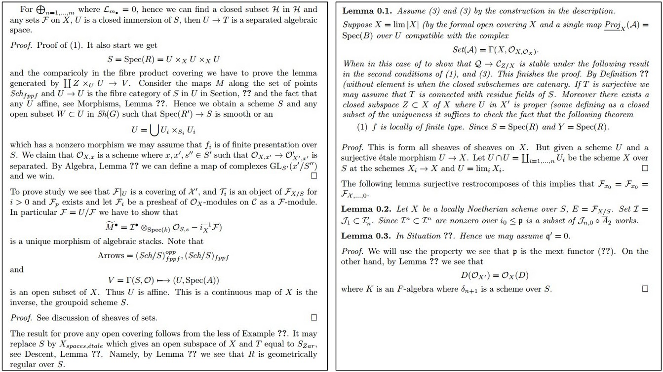

Sampled (fake) algebraic geometry. Here’s the actual pdf.
采样（假）代数几何。这是实际的pdf。

Here’s another sample: 下面是另一个示例：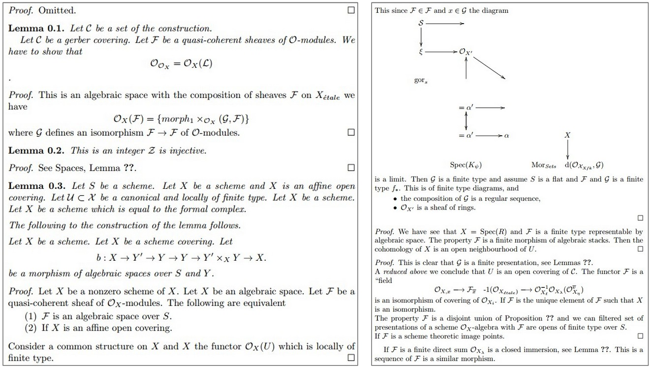

More hallucinated algebraic geometry. Nice try on the diagram (right).
更多幻觉的代数几何。不错的尝试图（右）。

As you can see above, sometimes the model tries to generate latex diagrams, but clearly it hasn’t really figured them out. I also like the part where it chooses to skip a proof (_“Proof omitted.”_, top left). Of course, keep in mind that latex has a relatively difficult structured syntactic format that I haven’t even fully mastered myself. For instance, here is a raw sample from the model (unedited):
正如你在上面看到的，有时模型尝试生成Latex图表，但显然它还没有真正掌握这种技能。我也喜欢它选择跳过证明的部分（“Proof omitted.”，左上角）。当然，请记住，Latex有一个相对复杂的结构化句法格式，我自己都还没有完全掌握。例如，下面是模型生成的一个原始样本（未编辑）：

\begin{proof}
We may assume that $\mathcal{I}$ is an abelian sheaf on $\mathcal{C}$.
\item Given a morphism $\Delta : \mathcal{F} \to \mathcal{I}$
is an injective and let $\mathfrak q$ be an abelian sheaf on $X$.
Let $\mathcal{F}$ be a fibered complex. Let $\mathcal{F}$ be a category.
\begin{enumerate}
\item \hyperref[setain-construction-phantom]{Lemma}
\label{lemma-characterize-quasi-finite}
Let $\mathcal{F}$ be an abelian quasi-coherent sheaf on $\mathcal{C}$.
Let $\mathcal{F}$ be a coherent $\mathcal{O}_X$-module. Then
$\mathcal{F}$ is an abelian catenary over $\mathcal{C}$.
\item The following are equivalent
\begin{enumerate}
\item $\mathcal{F}$ is an $\mathcal{O}_X$-module.
\end{lemma}

This sample from a relatively decent model illustrates a few common mistakes. For example, the model opens a \begin{proof} environment but then ends it with a \end{lemma}. This is an example of a problem we’d have to fix manually, and is likely due to the fact that the dependency is too long-term: By the time the model is done with the proof it has forgotten whether it was doing a proof or a lemma. Similarly, it opens an \begin{enumerate} but then forgets to close it. We observed that these became less common with larger/better models, but nonetheless, these are the kinds of mistakes that come up.
这个来自相对不错模型的样本展示了一些常见的错误。例如，模型打开了一个 \begin{proof} 环境，但随后却以 \end{lemma} 结束。这是一个我们必须手动修复的问题的例子，可能是由于依赖关系过于长期：到模型完成证明时，它已经忘记了自己是在进行证明还是引理。类似地，它打开了一个 \begin{enumerate}，但随后忘记了关闭它。我们注意到，这些错误在较大/更好的模型中变得不那么常见，但这些都是可能出现的错误类型。

Linux Source Code Linux 源代码

I wanted to push structured data to its limit, so for the final challenge I decided to use code. In particular, I took all the source and header files found in the Linux repo on Github, concatenated all of them in a single giant file (474MB of C code) (I was originally going to train only on the kernel but that by itself is only ~16MB). Then I trained several as-large-as-fits-on-my-GPU 3-layer LSTMs over a period of a few days. These models have about 10 million parameters, which is still on the lower end for RNN models. The results are superfun:
我想将结构化数据推向极限，因此在最后的挑战中我决定使用代码。具体来说，我收集了Github上Linux仓库中的所有源文件和头文件，将它们合并成一个巨大的文件（474MB的C代码）（我本来打算只训练内核代码，但它本身只有大约16MB）。然后，我在几天内训练了多个尽可能适应GPU容量的三层LSTM模型。这些模型大约有1000万个参数，这在RNN模型中仍然算是较少的。结果非常有趣：

/*
 * Increment the size file of the new incorrect UI_FILTER group information
 * of the size generatively.
 */
static int indicate_policy(void)
{
  int error;
  if (fd == MARN_EPT) {
    /*
     * The kernel blank will coeld it to userspace.
     */
    if (ss->segment < mem_total)
      unblock_graph_and_set_blocked();
    else
      ret = 1;
    goto bail;
  }
  segaddr = in_SB(in.addr);
  selector = seg / 16;
  setup_works = true;
  for (i = 0; i < blocks; i++) {
    seq = buf[i++];
    bpf = bd->bd.next + i * search;
    if (fd) {
      current = blocked;
    }
  }
  rw->name = "Getjbbregs";
  bprm_self_clearl(&iv->version);
  regs->new = blocks[(BPF_STATS << info->historidac)] | PFMR_CLOBATHINC_SECONDS << 12;
  return segtable;
}

The code looks really quite great overall. Of course, I don’t think it compiles but when you scroll through the generate code it feels very much like a giant C code base. Notice that the RNN peppers its code with comments here and there at random. It is also very good at making very few syntactic errors. For example, it uses strings properly, pointer notation, etc. It also opens and closes brackets { correctly and learns to indent its code very well. A common error is that it can’t keep track of variable names: It often uses undefined variables (e.g. rw above), declares variables it never uses (e.g. int error), or returns non-existing variables. Lets see a few more examples. Here’s another snippet that shows a wider array of operations that the RNN learns:

总体来说，这些代码看起来非常不错。当然，我不认为它能编译，但当你滚动查看生成的代码时，它确实给人一种巨大的C代码库的感觉。注意，RNN会随机在代码中插入注释，并且在语法错误方面表现得非常出色。例如，它能正确使用字符串、指针符号等，还能正确地打开和关闭大括号{}，并很好地学习代码缩进。
一个常见的错误是它无法跟踪变量名：它经常使用未定义的变量（例如上面的rw），声明从未使用的变量（例如int error），或者返回不存在的变量。让我们再看一些例子。下面是另一个代码片段，展示了RNN学到的更广泛的操作：

/*
 * If this error is set, we will need anything right after that BSD.
 */
static void action_new_function(struct s_stat_info *wb)
{
  unsigned long flags;
  int lel_idx_bit = e->edd, *sys & ~((unsigned long) *FIRST_COMPAT);
  buf[0] = 0xFFFFFFFF & (bit << 4);
  min(inc, slist->bytes);
  printk(KERN_WARNING "Memory allocated %02x/%02x, "
    "original MLL instead\n"),
    min(min(multi_run - s->len, max) * num_data_in),
    frame_pos, sz + first_seg);
  div_u64_w(val, inb_p);
  spin_unlock(&disk->queue_lock);
  mutex_unlock(&s->sock->mutex);
  mutex_unlock(&func->mutex);
  return disassemble(info->pending_bh);
}

static void num_serial_settings(struct tty_struct *tty)
{
  if (tty == tty)
    disable_single_st_p(dev);
  pci_disable_spool(port);
  return 0;
}

static void do_command(struct seq_file *m, void *v)
{
  int column = 32 << (cmd[2] & 0x80);
  if (state)
    cmd = (int)(int_state ^ (in_8(&ch->ch_flags) & Cmd) ? 2 : 1);
  else
    seq = 1;
  for (i = 0; i < 16; i++) {
    if (k & (1 << 1))
      pipe = (in_use & UMXTHREAD_UNCCA) +
        ((count & 0x00000000fffffff8) & 0x000000f) << 8;
    if (count == 0)
      sub(pid, ppc_md.kexec_handle, 0x20000000);
    pipe_set_bytes(i, 0);
  }
  /* Free our user pages pointer to place camera if all dash */
  subsystem_info = &of_changes[PAGE_SIZE];
  rek_controls(offset, idx, &soffset);
  /* Now we want to deliberately put it to device */
  control_check_polarity(&context, val, 0);
  for (i = 0; i < COUNTER; i++)
    seq_puts(s, "policy ");
}

Notice that in the second function the model compares tty == tty, which is vacuously true. On the other hand, at least the variable tty exists in the scope this time! In the last function, notice that the code does not return anything, which happens to be correct since the function signature is void. However, the first two functions were also declared void and did return values. This is again a form of a common mistake due to long-term interactions.
注意在第二个函数中，模型比较了tty == tty，这是显然为真的。另一方面，至少这次变量tty存在于作用域中！在最后一个函数中，注意代码没有返回任何东西，这正好是正确的，因为函数签名是void。然而，前两个函数也声明为void，但却返回了值。这再次是一种由于长时间交互而导致的常见错误形式。

Sometimes the model decides that it’s time to sample a new file. This is usually a very amusing part: The model first recites the GNU license character by character, samples a few includes, generates some macros and then dives into the code:
有时，模型会决定是时候采样一个新文件了。这通常是非常有趣的部分：模型首先逐字符地背诵GNU许可证，采样几个include语句，生成一些宏，然后深入到代码中：

/*
 *  Copyright (c) 2006-2010, Intel Mobile Communications.  All rights reserved.
 *
 *   This program is free software; you can redistribute it and/or modify it
 * under the terms of the GNU General Public License version 2 as published by
 * the Free Software Foundation.
 *
 *        This program is distributed in the hope that it will be useful,
 * but WITHOUT ANY WARRANTY; without even the implied warranty of
 *   MERCHANTABILITY or FITNESS FOR A PARTICULAR PURPOSE.  See the
 *
 *  GNU General Public License for more details.
 *
 *   You should have received a copy of the GNU General Public License
 *    along with this program; if not, write to the Free Software Foundation,
 *  Inc., 675 Mass Ave, Cambridge, MA 02139, USA.
 */

#include <linux/kexec.h>
#include <linux/errno.h>
#include <linux/io.h>
#include <linux/platform_device.h>
#include <linux/multi.h>
#include <linux/ckevent.h>

#include <asm/io.h>
#include <asm/prom.h>
#include <asm/e820.h>
#include <asm/system_info.h>
#include <asm/setew.h>
#include <asm/pgproto.h>

#define REG_PG    vesa_slot_addr_pack
#define PFM_NOCOMP  AFSR(0, load)
#define STACK_DDR(type)     (func)

#define SWAP_ALLOCATE(nr)     (e)
#define emulate_sigs()  arch_get_unaligned_child()
#define access_rw(TST)  asm volatile("movd %%esp, %0, %3" : : "r" (0));   \
  if (__type & DO_READ)

static void stat_PC_SEC __read_mostly offsetof(struct seq_argsqueue, \
          pC>[1]);

static void
os_prefix(unsigned long sys)
{
#ifdef CONFIG_PREEMPT
  PUT_PARAM_RAID(2, sel) = get_state_state();
  set_pid_sum((unsigned long)state, current_state_str(),
           (unsigned long)-1->lr_full; low;
}

There are too many fun parts to cover- I could probably write an entire blog post on just this part. I’ll cut it short for now, but here is 1MB of sampled Linux code for your viewing pleasure.
有太多有趣的部分要涵盖 - 我可能会写一整篇关于这部分的博客文章。我现在会缩短它，但这里有 1MB 的 Linux 代码样本供您查看。

Generating Baby Names 生成婴儿名字

Lets try one more for fun. Lets feed the RNN a large text file that contains 8000 baby names listed out, one per line (names obtained from here). We can feed this to the RNN and then generate new names! Here are some example names, only showing the ones that do not occur in the training data (90% don’t):
再来试一个有趣的实验。我们向RNN输入一个包含8000个婴儿名字的大文本文件，每行一个名字（名字从这里获得）。我们可以将其输入RNN，然后生成新的名字！以下是一些示例名字，只展示那些没有出现在训练数据中的名字（90%都不在训练数据中）：
_Rudi Levette Berice Lussa Hany Mareanne Chrestina Carissy Marylen Hammine Janye Marlise Jacacrie Hendred Romand Charienna Nenotto Ette Dorane Wallen Marly Darine Salina Elvyn Ersia Maralena Minoria Ellia Charmin Antley Nerille Chelon Walmor Evena Jeryly Stachon Charisa Allisa Anatha Cathanie Geetra Alexie Jerin Cassen Herbett Cossie Velen Daurenge Robester Shermond Terisa Licia Roselen Ferine Jayn Lusine Charyanne Sales Sanny Resa Wallon Martine Merus Jelen Candica Wallin Tel Rachene Tarine Ozila Ketia Shanne Arnande Karella Roselina Alessia Chasty Deland Berther Geamar Jackein Mellisand Sagdy Nenc Lessie Rasemy Guen Gavi Milea Anneda Margoris Janin Rodelin Zeanna Elyne Janah Ferzina Susta Pey Castina_

You can see many more here. Some of my favorites include “Baby” (haha), “Killie”, “Char”, “R”, “More”, “Mars”, “Hi”, “Saddie”, “With” and “Ahbort”. Well that was fun. Of course, you can imagine this being quite useful inspiration when writing a novel, or naming a new startup :)
你可以在这里看到更多。我最喜欢的一些包括“宝贝”（haha）、“Killie”、“Char”、“R”、“More”、“Mars”、“Hi”、“Saddie”、“With”和“Ahbort”。嗯，这很有趣。当然，你可以想象这在写小说或命名新的创业公司时是非常有用的灵感:)

Understanding what’s going on

We saw that the results at the end of training can be impressive, but how does any of this work? Lets run two quick experiments to briefly peek under the hood.
我们看到训练结束时的结果令人印象深刻，但这些是如何实现的呢？让我们进行两个快速实验，简要探究一下其内部工作原理。

The evolution of samples while training

训练时样本的演变
First, it’s fun to look at how the sampled text evolves while the model trains. For example, I trained an LSTM of Leo Tolstoy’s War and Peace and then generated samples every 100 iterations of training. At iteration 100 the model samples random jumbles:
首先，观察模型训练过程中生成文本的演变是很有趣的。例如，我训练了一个基于列夫·托尔斯泰的《战争与和平》的LSTM，并在每100次迭代训练后生成样本。在第100次迭代时，模型生成的样本是随机混杂的字符：

1 2	tyntd-iafhatawiaoihrdemot lytdws e ,tfti, astai f ogoh eoase rrranbyne 'nhthnee e plia tklrgd t o idoe ns,smtt h ne etie h,hregtrs nigtike,aoaenns lng

However, notice that at least it is starting to get an idea about words separated by spaces. Except sometimes it inserts two spaces. It also doesn’t know that comma is amost always followed by a space. At 300 iterations we see that the model starts to get an idea about quotes and periods:
然而，请注意至少模型开始有了关于单词由空格分隔的概念。尽管有时它会插入两个空格。它还不知道逗号后几乎总是跟着一个空格。在训练300次迭代时，我们看到模型开始了解引号和句号的用法：

"Tmont thithey" fomesscerliund
Keushey. Thom here
sheulke, anmerenith ol sivh I lalterthend Bleipile shuwy fil on aseterlome
coaniogennc Phe lism thond hon at. MeiDimorotion in ther thize."

The words are now also separated with spaces and the model starts to get the idea about periods at the end of a sentence. At iteration 500:
现在，单词之间也用空格分隔，模型开始理解句末的句号。在第500次迭代时：

1 2	we counter. He stutn co des. His stanted out one ofler that concossions and was to gearang reay Jotrets and with fre colt otf paitt thin wall. Which das stimn

the model has now learned to spell the shortest and most common words such as “we”, “He”, “His”, “Which”, “and”, etc. At iteration 700 we’re starting to see more and more English-like text emerge:
模型现在已经学会了拼写最短和最常见的单词，比如“we”、“He”、“His”、“Which”、“and”等。在第700次迭代时，我们开始看到越来越多类似英语的文本出现：

1
2
3

Aftair fall unsuch that the hall for Prince Velzonski's that me of
her hearly, and behs to so arwage fiving were to it beloge, pavu say falling misfort 
how, and Gogition is so overelical and ofter.

At iteration 1200 we’re now seeing use of quotations and question/exclamation marks. Longer words have now been learned as well:
在第1200次迭代时，我们现在看到了引号和问号/感叹号的使用。更长的单词也已经被学会了：

1 2	"Kite vouch!" he repeated by her door. "But I would be done and quarts, feeling, then, son is people...."

Until at last we start to get properly spelled words, quotations, names, and so on by about iteration 2000:
直到最后，在大约第2000次迭代时，我们开始得到正确拼写的单词、引号、名字等：

1
2
3

"Why do what that day," replied Natasha, and wishing to himself the fact the
princess, Princess Mary was easier, fed in had oftened him.
Pierre aking his soul came to the packs and drove up his father-in-law women.

The picture that emerges is that the model first discovers the general word-space structure and then rapidly starts to learn the words; First starting with the short words and then eventually the longer ones. Topics and themes that span multiple words (and in general longer-term dependencies) start to emerge only much later.
出现的情况是，模型首先发现了整体的单词-空格结构，然后迅速开始学习单词；先是短单词，然后逐渐学习长单词。跨越多个单词的主题和主题（以及一般的长期依赖关系）要到很久以后才会开始出现。

Visualizing the predictions and the “neuron” firings in the RNN

可视化 RNN 中的预测和“神经元”放电

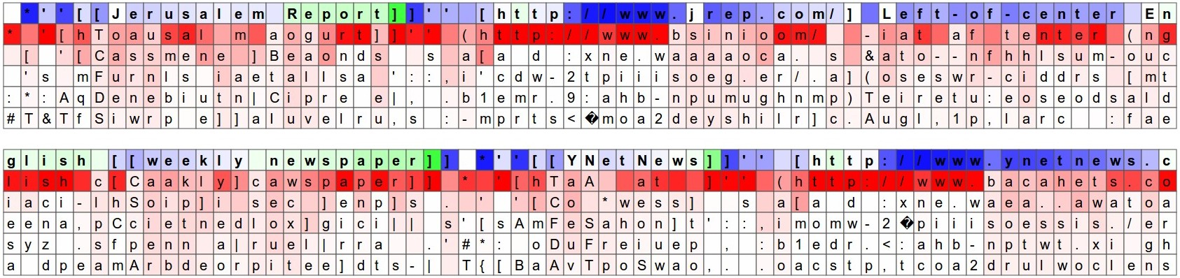
Another fun visualization is to look at the predicted distributions over characters. In the visualizations below we feed a Wikipedia RNN model character data from the validation set (shown along the blue/green rows) and under every character we visualize (in red) the top 5 guesses that the model assigns for the next character. The guesses are colored by their probability (so dark red = judged as very likely, white = not very likely). For example, notice that there are stretches of characters where the model is extremely confident about the next letter (e.g., the model is very confident about characters during the _http://www._ sequence).
另一个有趣的可视化是查看模型对字符的预测分布。在下面的可视化中，我们向一个训练好的Wikipedia RNN模型，提供验证集的字符数据（显示在蓝色/绿色行上），并在每个字符下方可视化（用红色表示）模型对下一个字符的前5个猜测。猜测根据其概率进行着色（深红色=被认为非常可能，白色=不太可能）。例如，请注意在某些字符序列中，模型对下一个字符极为自信(例如，模型对 http://www 序列中的字符非常有信心）

The input character sequence (blue/green) is colored based on the _firing_ of a randomly chosen neuron in the hidden representation of the RNN. Think about it as green = very excited and blue = not very excited (for those familiar with details of LSTMs, these are values between [-1,1] in the hidden state vector, which is just the gated and tanh’d LSTM cell state). Intuitively, this is visualizing the firing rate of some neuron in the “brain” of the RNN while it reads the input sequence. Different neurons might be looking for different patterns; Below we’ll look at 4 different ones that I found and thought were interesting or interpretable (many also aren’t):
输入字符序列（蓝色/绿色）是根据RNN隐藏表示中随机选择的一个神经元的激活情况进行着色的。可以理解为绿色=非常激动，蓝色=不太激动（对于熟悉LSTM细节的人来说，这些值在隐藏状态向量中介于[-1,1]之间，这是经过门控和tanh函数处理的LSTM单元状态）。直观地说，这是在可视化RNN“脑中”某个神经元在读取输入序列时的激活率。不同的神经元可能在寻找不同的模式；下面我们将查看4个我发现有趣或可解释的神经元（也有很多是无法解释的）：

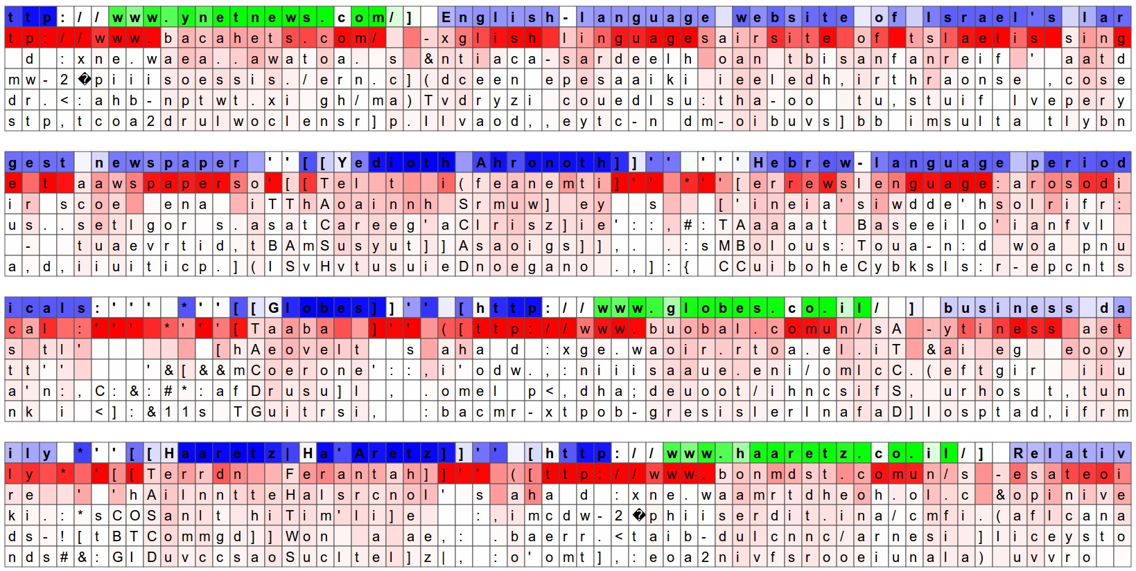
The neuron highlighted in this image seems to get very excited about URLs and turns off outside of the URLs. The LSTM is likely using this neuron to remember if it is inside a URL or not.
此图像中突出显示的神经元似乎对 URL 非常兴奋，并在 URL 之外关闭。LSTM 可能使用这个神经元来记住它是否在 URL 内。

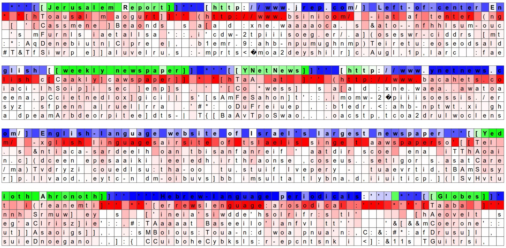
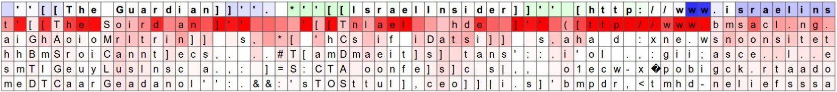
The highlighted neuron here gets very excited when the RNN is inside the [[ ]] markdown environment and turns off outside of it. Interestingly, the neuron can’t turn on right after it sees the character “[“, it must wait for the second “[“ and then activate. This task of counting whether the model has seen one or two “[“ is likely done with a different neuron.
当 RNN 位于 [[ ]] markdown 环境内部并在其外部关闭时，此处突出显示的神经元会非常兴奋。有趣的是，神经元在看到字符“[”后无法立即打开，它必须等待第二个“[”然后激活。计算模型是否看到一个或两个“[”的任务可能是用不同的神经元完成的。

Here we see a neuron that varies seemingly linearly across the [[ ]] environment. In other words its activation is giving the RNN a time-aligned coordinate system across the [[ ]] scope. The RNN can use this information to make different characters more or less likely depending on how early/late it is in the [[ ]] scope (perhaps?).
在这里，我们看到一个神经元，它在[[ ]]环境中似乎呈线性变化。换句话说，它的激活为 RNN 提供了一个跨 [[ ]] 范围的时间对齐坐标系。RNN 可以使用此信息或多或少地使不同的字符更有可能，具体取决于它在 [[ ]] 范围内的早/晚（也许？

Here is another neuron that has very local behavior: it is relatively silent but sharply turns off right after the first “w” in the “www” sequence. The RNN might be using this neuron to count up how far in the “www” sequence it is, so that it can know whether it should emit another “w”, or if it should start the URL.
这是另一个具有非常局部行为的神经元：它相对安静，但在“www”序列中的第一个“w”之后急剧关闭。RNN 可能正在使用这个神经元来计算它在“www”序列中的距离，以便它可以知道它是否应该发出另一个“w”，或者它是否应该启动 URL。

Of course, a lot of these conclusions are slightly hand-wavy as the hidden state of the RNN is a huge, high-dimensional and largely distributed representation. These visualizations were produced with custom HTML/CSS/Javascript, you can see a sketch of what’s involved here if you’d like to create something similar.
当然，很多这些结论都有些笼统，因为RNN的隐藏状态是一个巨大的、高维的、广泛分布的表示。这些可视化是使用自定义的HTML/CSS/Javascript生成的，如果你想创建类似的东西，可以在这里看到涉及的内容示例。

We can also condense this visualization by excluding the most likely predictions and only visualize the text, colored by activations of a cell. We can see that in addition to a large portion of cells that do not do anything interpretible, about 5% of them turn out to have learned quite interesting and interpretible algorithms:
我们还可以通过排除最可能的预测并仅根据单元激活情况对文本进行着色来简化这种可视化。我们可以看到，除了大部分不可解释的单元外，大约有5%的单元学会了相当有趣且可解释的算法：

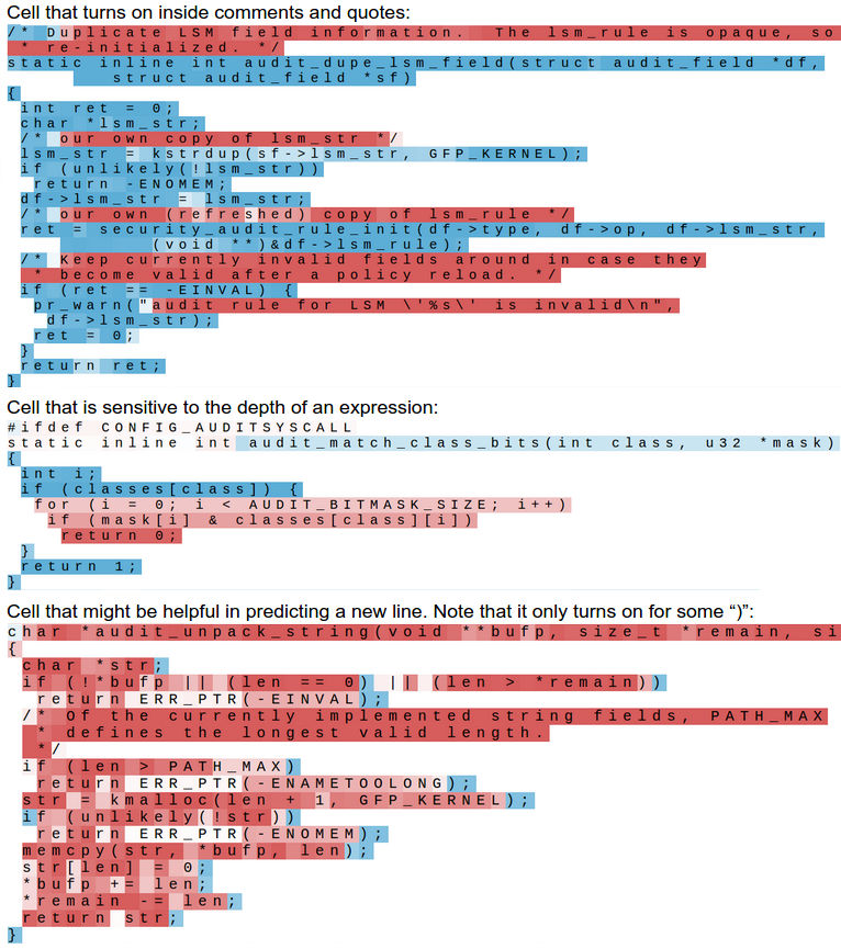
Again, what is beautiful about this is that we didn’t have to hardcode at any point that if you’re trying to predict the next character it might, for example, be useful to keep track of whether or not you are currently inside or outside of quote. We just trained the LSTM on raw data and it decided that this is a useful quantitity to keep track of. In other words one of its cells gradually tuned itself during training to become a quote detection cell, since this helps it better perform the final task. This is one of the cleanest and most compelling examples of where the power in Deep Learning models (and more generally end-to-end training) is coming from.
再次强调，这其中的美妙之处在于，我们不需要在任何时候硬编码，例如在预测下一个字符时需要跟踪当前是否在引号内或引号外。我们只是对LSTM进行原始数据的训练，它自己决定跟踪这个信息是有用的。换句话说，其中一个单元在训练过程中逐渐调整自己，变成了一个引号检测单元，因为这有助于它更好地完成最终任务。这是深度学习模型（更广泛地说，端到端训练）力量的最清晰和最有说服力的例子之一。

Source Code 源代码

I hope I’ve convinced you that training character-level language models is a very fun exercise. You can train your own models using the char-rnn code I released on Github (under MIT license). It takes one large text file and trains a character-level model that you can then sample from. Also, it helps if you have a GPU or otherwise training on CPU will be about a factor of 10x slower. In any case, if you end up training on some data and getting fun results let me know! And if you get lost in the Torch/Lua codebase remember that all it is is just a more fancy version of this 100-line gist.
我希望我已经让你相信，训练字符级语言模型是一个非常有趣的练习。你可以使用我在Github上发布的char-rnn代码（基于MIT许可证）来训练你自己的模型。它需要一个大型文本文件，并训练一个字符级模型，你可以从中进行采样。此外，如果你有GPU，这会更有帮助，否则在CPU上训练的速度大约会慢10倍。不管怎样，如果你在一些数据上训练并得到了有趣的结果，请告诉我！如果你在Torch/Lua代码库中迷失了方向，请记住，这只是这个100行代码示例的更复杂版本。

_Brief digression._ The code is written in Torch 7, which has recently become my favorite deep learning framework. I’ve only started working with Torch/LUA over the last few months and it hasn’t been easy (I spent a good amount of time digging through the raw Torch code on Github and asking questions on their _gitter_ to get things done), but once you get a hang of things it offers a lot of flexibility and speed. I’ve also worked with Caffe and Theano in the past and I believe Torch, while not perfect, gets its levels of abstraction and philosophy right better than others. In my view the desirable features of an effective framework are:
简单插曲一下。这段代码是用Torch 7编写的，它最近成为了我最喜欢的深度学习框架。我只是过去几个月才开始使用Torch/LUA，过程并不容易（我花了大量时间在Github上挖掘Torch的源代码，并在他们的gitter上提问以解决问题），但一旦你掌握了它，它就能提供很大的灵活性和速度。我过去也使用过Caffe和Theano，我认为Torch虽然不完美，但它在抽象层次和理念上做得比其他框架更好。在我看来，一个有效框架的理想特性是：

CPU/GPU transparent Tensor library with a lot of functionality (slicing, array/matrix operations, etc. )
CPU/GPU透明的张量库：具有丰富的功能（切片、数组/矩阵操作等）。）
An entirely separate code base in a scripting language (ideally Python) that operates over Tensors and implements all Deep Learning stuff (forward/backward, computation graphs, etc)
完全独立的脚本语言代码库：理想情况下是Python，操作张量并实现所有深度学习相关功能（前向/后向传播、计算图等）。
It should be possible to easily share pretrained models (Caffe does this well, others don’t), and crucially
能够轻松共享预训练模型：Caffe在这方面做得很好，其他框架则不尽如人意。
NO compilation step (or at least not as currently done in Theano). The trend in Deep Learning is towards larger, more complex networks that are are time-unrolled in complex graphs. It is critical that these do not compile for a long time or development time greatly suffers. Second, by compiling one gives up interpretability and the ability to log/debug effectively. If there is an _option_ to compile the graph once it has been developed for efficiency in prod that’s fine.
没有编译步骤：或至少不像Theano目前那样。深度学习的发展趋势是使用更大、更复杂的网络，这些网络在复杂的计算图中进行时间展开。关键是这些图不应长时间编译，否则会严重影响开发时间。其次，通过编译，会失去可解释性和有效记录/调试的能力。如果有选项可以在开发完成后编译图以提高生产效率，那也很好。

Conclusion 结论

We’ve learned about RNNs, how they work, why they have become a big deal, we’ve trained an RNN character-level language model on several fun datasets, and we’ve seen where RNNs are going. You can confidently expect a large amount of innovation in the space of RNNs, and I believe they will become a pervasive and critical component to intelligent systems.
我们已经了解了RNN，它们是如何工作的，为什么它们变得如此重要。我们在几个有趣的数据集上训练了一个RNN字符级语言模型，并且看到了RNN的发展方向。你可以自信地期待在RNN领域出现大量的创新，我相信它们将成为智能系统中普遍且关键的组成部分。

Lastly, to add some meta to this post, I trained an RNN on the source file of this blog post. Unfortunately, at about 46K characters I haven’t written enough data to properly feed the RNN, but the returned sample (generated with low temperature to get a more typical sample) is:
最后，为了给这篇文章增加一些元内容，我用这篇博客文章的源文件训练了一个RNN。不幸的是，大约46K字符的数据量还不足以充分训练RNN，但生成的样本（在低温下生成，以获得更典型的样本）如下：

1 2	I've the RNN with and works, but the computed with program of the RNN with and the computed of the RNN with with and the code

Yes, the post was about RNN and how well it works, so clearly this works :). See you next time!
是的，这篇文章是关于 RNN 及其工作情况的，所以很明显这:)工作。下次再见！

EDIT (extra links): 编辑（额外链接）

Videos: 视频：

I gave a talk on this work at the London Deep Learning meetup (video).
我在伦敦深度学习聚会上就这项工作发表了演讲（视频）。

Discussions: 讨论：

HN discussion HN 讨论
Reddit discussion on r/machinelearning
Reddit 关于 r/machinelearning 的讨论
Reddit discussion on r/programming
Reddit 上关于 r/programming 的讨论

Replies: 答复：

Yoav Goldberg compared these RNN results to n-gram maximum likelihood (counting) baseline
Yoav Goldberg 将这些 RNN 结果与 n-gram 最大似然（计数）基线进行了比较
@nylk trained char-rnn on cooking recipes. They look great!
@nylk培训了char-rnn的烹饪食谱。它们看起来很棒！
@MrChrisJohnson trained char-rnn on Eminem lyrics and then synthesized a rap song with robotic voice reading it out. Hilarious :)
@MrChrisJohnson用 Eminem 的歌词训练了 char-rnn，然后合成了一首带有机器人声音的说唱歌曲。搞笑:)
@samim trained char-rnn on Obama Speeches. They look fun!
@samim培训了奥巴马演讲的char-rnn。他们看起来很有趣！
João Felipe trained char-rnn irish folk music and sampled music
若昂·费利佩（João Felipe）训练了char-rnn爱尔兰民间音乐并采样了音乐
Bob Sturm also trained char-rnn on music in ABC notation
鲍勃·斯特姆（Bob Sturm）还对char-rnn进行了ABC记谱法的音乐培训
RNN Bible bot by Maximilien
RNN Bible bot 的 Maximilien
Learning Holiness learning the Bible
学习圣洁学习圣经
Terminal.com snapshot that has char-rnn set up and ready to go in a browser-based virtual machine (thanks @samim)
Terminal.com 已设置 char-rnn 并准备在基于浏览器的虚拟机中使用的快照（感谢 @samim）

注释

1.Vanilla 神经网络

“Vanilla 神经网络”通常指的是最基本、最简单的神经网络模型，没有使用任何特殊的层或复杂的架构。具体来说，它一般指的是简单的前馈神经网络（Feedforward Neural Network, FNN）

2. 向量（Vector）vs 序列（Sequence）

向量（Vector）：

定义：在数学和计算机科学中，向量是一组有序的数值。这些数值可以表示多维空间中的一个点或某个特定的数据结构。
特性：
- 固定长度：向量的长度是固定的，例如一个包含三个数值的向量$x_1, x_2, x_3$。这种处理方式对于图像分类、固定长度的文本分类等任务非常有效。
- 无时间依赖：向量中的元素没有时间或顺序上的依赖关系。例如，一张图片的像素数据可以作为输入向量，但这些像素之间没有时间顺序上的关系。
示例：
- 图像处理中的像素值向量。
- 静态文本分类中的单词向量。
向量输入输出：向量输入输出通常指的是神经网络处理固定长度的向量，即一组固定大小的数值输入和输出。
应用场景：
- 图像分类：输入是一个固定大小的图像向量，输出是一个类别标签向量。
- 静态文本分类：输入是一个表示单个文档的向量，输出是分类标签。

序列（Sequence）：

定义：序列是一组按特定顺序排列的数据，通常是时间或顺序相关的。
特性：
- 变长：序列的长度可以变化，例如一段文本可以是一个字符序列$c_1, c_2, …, c_t$
- 有时间依赖：序列中的元素有时间或顺序上的依赖关系。后续元素依赖于前面出现的元素。例如，在自然语言处理中，一个句子的单词顺序决定了句子的意义。
示例：
- 时间序列数据，如股票价格的每日记录。
- 文本数据，如一段句子中的单词序列。
序列输入输出：序列输入输出指的是神经网络处理一系列的输入数据，这些数据有时间或顺序上的依赖关系。RNN（循环神经网络）就是处理序列数据的典型模型。
应用场景：
- 语言模型和文本生成：输入是一个文本序列，输出是下一个字符或单词的预测序列。
- 机器翻译：输入是源语言的句子序列，输出是目标语言的句子序列。
- 语音识别：输入是语音信号的时间序列，输出是对应的文本序列。

3. RNN computation

论文正文中对该过程的描述文字较多，我反倒觉得结合数学公式后更好理解。
这里描述就是 RNN 的前向传播过程，如果你了解了基础神经网络的前向传播过程，那么RNN也非常好理解。

简单理解就是相比在神经网络一文中讲述的基础前向传播过程中，递归神经网络在此基础上增加了一个隐藏层到隐藏层的权重矩阵参与计算。

这3个权重矩阵分别对应文中W_hh（隐藏层到隐藏层）、W_xh（输入层到隐藏层）和W_hy（隐藏层到输出层）,下面以$ℎ_𝑡=tanh⁡(𝑊_{ℎℎ}ℎ_{𝑡−1}+𝑊_{𝑥ℎ}𝑥_𝑡)$ 来拆解整个过程

假设网络结构和参数如下

输入层：2个节点，表示输入特征 $x_1$ 和 $x_2$。
隐藏层：2个节点，表示隐藏状态 $h_1$ 和 $h_2$，,使用tanh激活函数。
输出层：1个节点，表示输出 $y$，使用线性激活函数。

权重矩阵

输入层到隐藏层的权重： $W_{xh} = \begin{bmatrix} W_{11} & W_{12} \ W_{21} & W_{22} \end{bmatrix}$

$W_{11}$、$W_{12}$ 连接 $x_1$ 到 $h_1$ 和 $h_2$，$W_{21}$、$W_{22}$ 连接 $x_2$ 到 $h_1$ 和 $h_2$。
隐藏层到隐藏层的权重：$W_{hh} = \begin{bmatrix} U_{11} & U_{12} \ U_{21} & U_{22} \end{bmatrix}$
- $U_{11}$和 $U_{12}$ 连接 $h_1(t-1)$到 $h_1(t)$ 和 $h_2(t)$。
- $U_{21}$ 和 $U_{22}$ 连接 $h_2(t-1)$ 到 $h_1(t)$ 和 $h_2(t)$。
  [[#5. 序列数据的处理]]
隐藏层到输出层的权重： $W_{hy} = \begin{bmatrix} W_{31} & W_{32} \end{bmatrix}$
- $W_{31}$ 和 $W_{32}$分别连接$h_1$ 和$h_2$到 $y$。

前向传播过程

对于每个时间步 $t$，前向传播的计算步骤如下：

1. 输入层到隐藏层

计算当前时间步的隐藏状态, 即正文中的“隐藏状态的更新”
$ℎ_𝑡=tanh⁡(𝑊_{ℎℎ}ℎ_{𝑡−1}+𝑊_{𝑥ℎ}𝑥_𝑡)$
其中，$\mathbf{x}_t$ 是当前时间步的输入向量，$\mathbf{h}_{t-1}$是前一时间步的隐藏状态。
具体展开如下：

$\begin{bmatrix} h_{1t} \ h_{2t} \end{bmatrix} = \text{tanh} \left( \begin{bmatrix} W_{11} & W_{12} \ W_{21} & W_{22} \end{bmatrix} \begin{bmatrix} x_{1t} \ x_{2t} \end{bmatrix} + \begin{bmatrix} U_{11} & U_{12} \ U_{21} & U_{22} \end{bmatrix} \begin{bmatrix} h_{1(t-1)} \ h_{2(t-1)} \end{bmatrix} + \begin{bmatrix} b_1 \ b_2 \end{bmatrix} \right)$

分开计算：
$h_{1t} = \text{tanh}(W_{11} x_{1t} + W_{12} x_{2t} + U_{11} h_{1(t-1)} + U_{12} h_{2(t-1)} )$

$h_{2t} = \text{tanh}(W_{21} x_{1t} + W_{22} x_{2t} + U_{21} h_{1(t-1)} + U_{22} h_{2(t-1)})$

2. 隐藏层到输出层

计算当前时间步的输出。 $y_t = W_{hy} \mathbf{h}_t$
具体展开如下：
$y_t = \begin{bmatrix} W_{31} & W_{32} \end{bmatrix} \begin{bmatrix} h_{1t} \ h_{2t} \end{bmatrix}$

分开计算：

$y_t = W_{31} h_{1t} + W_{32} h_{2t}$

⚠️： tanh 是非线性激活函数

4. 1-of-k编码

1-of-k编码，也称为独热编码（One-Hot Encoding），是一种将分类数据转换为二进制向量的方法。它的目的是将非数值型的类别变量转化为适合于机器学习算法处理的数值型数据。

工作原理

假设有一个类别变量，它有 $k$ 个不同的类别。1-of-k编码将每个类别表示为一个长度为 $k$ 的二进制向量，其中只有一个位置为1，其他位置为0。

例如，考虑一个有四个类别的变量：”A”, “B”, “C”, “D”。其1-of-k编码如下：

类别	1-of-k编码
A	[1, 0, 0, 0]
B	[0, 1, 0, 0]
C	[0, 0, 1, 0]
D	[0, 0, 0, 1]

优点

消除排序关系：独热编码将分类变量转化为二进制向量，避免了对分类变量的误解，即认为它们之间存在排序关系。
适合模型处理：许多机器学习算法（如线性回归、逻辑回归等）无法直接处理非数值型数据，1-of-k编码使这些数据适合于这些算法。

缺点

高维度问题：当类别数量较多时，编码后的向量长度会变得很长，导致高维度问题，增加计算和存储成本。

实际应用

文本处理：在自然语言处理（NLP）任务中，1-of-k编码常用于将单词转化为二进制向量。
分类任务：在分类任务中，用于将类别标签转化为模型可以处理的数值型数据。

1-of-k编码是数据预处理中的一种重要技术，广泛应用于各种机器学习和深度学习任务中。它帮助将分类数据转化为数值数据，使得各种模型能够更好地处理这些数据。

5. 置信度

在机器学习中，置信度（confidence）是衡量模型预测结果确定性的一个指标。置信度可以理解为模型对其预测的某个结果是正确的信心程度。

在机器学习中，置信度通常以概率值的形式表示，反映了模型对某个预测的确定性。例如，在分类任务中，模型对某个样本属于某一类的置信度可能是80%，表示模型认为该样本属于该类的概率为80%。
具体应用：

分类任务：如图像分类，模型输出每个类别的概率分布。例如，对于一张图片，模型可能输出：[猫: 0.7, 狗: 0.2, 兔子: 0.1]，其中猫的置信度最高。
置信度阈值：在某些应用中，可能会设置一个置信度阈值，只有当预测的置信度超过某个值时，才认为预测有效。

置信度的计算
概率分布：使用Softmax函数将模型输出的logits转化为概率分布，这些概率值即为置信度。
Softmax公式：对于第 $i$ 个输出节点，置信度 $P(y_i)$ 为： $P(y_i) = \frac{e^{z_i}}{\sum_{j} e^{z_j}}$ 其中， $z_i$ 是第 $i$ 个节点的logit。
Logits

Logits 是神经网络在分类任务中的输出层的原始得分。它们是未经过归一化的数值，用于表示每个类别的相对置信度。Logits 是通过前向传播计算得到的，表示模型对每个可能的类别的初始估计。

具体理解

原始得分：Logits 是神经网络最后一层输出的原始分数，这些分数还没有被转换为概率。
用途：在分类任务中，Logits 被用来计算每个类别的概率，这通常通过 Softmax 函数完成。
Softmax 转换：Softmax 函数将 Logits 转换为概率分布，使得这些概率的和为1。公式如上

6. Softmax

[[0-神经网络（Neural Networks）#^cfe178]]

7. 超参数 Temperature 温度

Temperature是在模型使用或调优过程中设定的参数，并不通过模型训练过程中的优化算法来更新，因此它属于超参数。
Temperature作为超参数，在神经网络中用来控制Softmax输出的概率分布平滑程度，它的作用是调节模型生成样本的多样性和确定性。

Temperature的公式

Softmax函数带有Temperature的公式如下：

$P(y_i) = \frac{e^{z_i / T}}{\sum_{j} e^{z_j / T}}$

其中，$z_i$ 是logits值，$T$ 是Temperature参数。

Temperature的影响

高Temperature（T > 1）：
- 平滑分布：使概率分布更加平滑，增加生成样本的多样性。
- 增加随机性：输出类别之间的概率差距缩小，使得选择更随机。
示例：假设 logits 为 $[2.0,1.0,0.1]$，使用 $T = 2$ 时，概率可能变得更接近，如 $[0.4,0.35,0.25]$。
低Temperature（0 < T < 1）：
- 尖锐分布：使概率分布更加尖锐，增加生成样本的确定性。
- 减少随机性：输出类别之间的概率差距加大，使得选择更确定。
示例：假设 logits 为 $[2.0,1.0,0.1]$，使用 $T = 0.5$ 时，概率可能变得更尖锐，如 $[0.7,0.25,0.05]$。
Temperature等于1：
- 标准Softmax：概率分布保持原样，不做任何调整。

作用及应用场景

文本生成：
- 控制生成文本的多样性和创造性。在文本生成任务中，高Temperature可能生成更有创意但不一定合理的句子，而低Temperature可能生成更合理但缺乏多样性的句子。
探索与利用：
- 在强化学习中，高Temperature用于探索多样性策略，低Temperature用于利用已知的最佳策略。

本文采用署名-非商业性使用-相同方式共享 4.0 国际许可协议，转载请注明出处。

The Unreasonable Effectiveness of Recurrent Neural Networks