Recurrent Neural Networks
递归神经网络
Humans don’t start their thinking from scratch every second. As you read this essay, you understand each word based on your understanding of previous words. You don’t throw everything away and start thinking from scratch again. Your thoughts have persistence.
人类不会每秒都从头开始思考。当你阅读这篇文章时,你会基于对之前词语的理解来理解每个词。你不会把所有东西都丢掉然后重新开始思考。你的思维是有连续性的。
Traditional neural networks can’t do this, and it seems like a major shortcoming. For example, imagine you want to classify what kind of event is happening at every point in a movie. It’s unclear how a traditional neural network could use its reasoning about previous events in the film to inform later ones.
传统的神经网络做不到这一点,这似乎是一个主要的缺陷。比如,想象一下你想对电影中每个时刻发生的事件类型进行分类。目前尚不清楚传统的神经网络如何利用其对电影中先前事件的推理来为后来的事件提供信息。
Recurrent neural networks address this issue. They are networks with loops in them, allowing information to persist.
循环神经网络解决了这个问题。它们是内部带有循环的网络,允许信息持续存在。
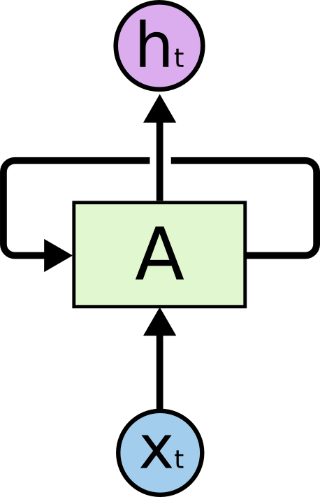
Recurrent Neural Networks have loops. 递归神经网络有循环。
In the above diagram, a chunk of neural network, 𝐴, looks at some input $𝑥_𝑡$ and outputs a value $ℎ_𝑡$. A loop allows information to be passed from one step of the network to the next.
在上图中,神经网络的一部分 $A$ ,查看一些输入$x_t$ 并输出一个值 $h_t$。一个循环允许信息从网络的一个步骤传递到下一个步骤。
These loops make recurrent neural networks seem kind of mysterious. However, if you think a bit more, it turns out that they aren’t all that different than a normal neural network. A recurrent neural network can be thought of as multiple copies of the same network, each passing a message to a successor. Consider what happens if we unroll the loop:
这些循环使循环神经网络看起来有点神秘。然而,如果你多想一点,就会发现它们与普通的神经网络并没有太大的不同。递归神经网络可以被认为是同一网络的多个副本,每个副本将消息传递给继任者。考虑一下如果我们展开循环会发生什么: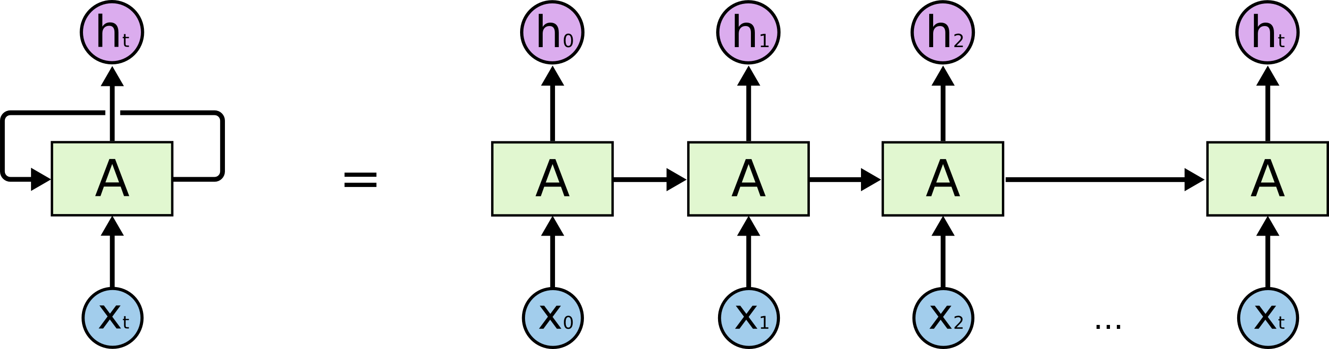
An unrolled recurrent neural network. 展开的循环神经网络。
This chain-like nature reveals that recurrent neural networks are intimately related to sequences and lists. They’re the natural architecture of neural network to use for such data.
这种链式结构表明,递归神经网络与序列和列表密切相关。它们是处理此类数据的自然神经网络架构。
And they certainly are used! In the last few years, there have been incredible success applying RNNs to a variety of problems: speech recognition, language modeling, translation, image captioning… The list goes on. I’ll leave discussion of the amazing feats one can achieve with RNNs to Andrej Karpathy’s excellent blog post, The Unreasonable Effectiveness of Recurrent Neural Networks. But they really are pretty amazing.
他们当然被使用了!在过去的几年里,将RNN应用于各种问题取得了令人难以置信的成功:语音识别、语言建模、翻译、图像字幕……这样的例子不胜枚举。我将把关于RNN可以实现的惊人壮举的讨论留给Andrej Karpathy的优秀博客文章,递归神经网络的不合理有效性。但他们真的非常了不起。
Essential to these successes is the use of “LSTMs,” a very special kind of recurrent neural network which works, for many tasks, much much better than the standard version. Almost all exciting results based on recurrent neural networks are achieved with them. It’s these LSTMs that this essay will explore.
这些成功的关键是“LSTM”的使用,这是一种非常特殊的递归神经网络,对于许多任务,它比标准版本要好得多。几乎所有基于递归神经网络的令人兴奋的结果都是通过它们实现的。本文将探讨的正是这些 LSTM。
The Problem of Long-Term Dependencies
长期依赖性问题
One of the appeals of RNNs is the idea that they might be able to connect previous information to the present task, such as using previous video frames might inform the understanding of the present frame. If RNNs could do this, they’d be extremely useful. But can they? It depends.
RNN的吸引力之一是,它们可能能够将先前的信息与当前任务联系起来,例如使用以前的视频帧可能会为理解当前帧提供信息。如果RNN可以做到这一点,它们将非常有用。但是他们能做到吗?这要视情况而定。
Sometimes, we only need to look at recent information to perform the present task. For example, consider a language model trying to predict the next word based on the previous ones. If we are trying to predict the last word in “the clouds are in the _sky_,” we don’t need any further context – it’s pretty obvious the next word is going to be sky. In such cases, where the gap between the relevant information and the place that it’s needed is small, RNNs can learn to use the past information.
有时候,我们只需要查看最近的信息就可以完成当前的任务。例如,考虑一个语言模型,它尝试基于前面的单词来预测下一个单词。如果我们试图预测“the clouds are in the sky”中的最后一个单词,我们不需要任何进一步的上下文——很明显下一个单词将是sky。在这种情况下,相关信息和所需位置之间的间隔较小,RNNs可以学习使用过去的信息。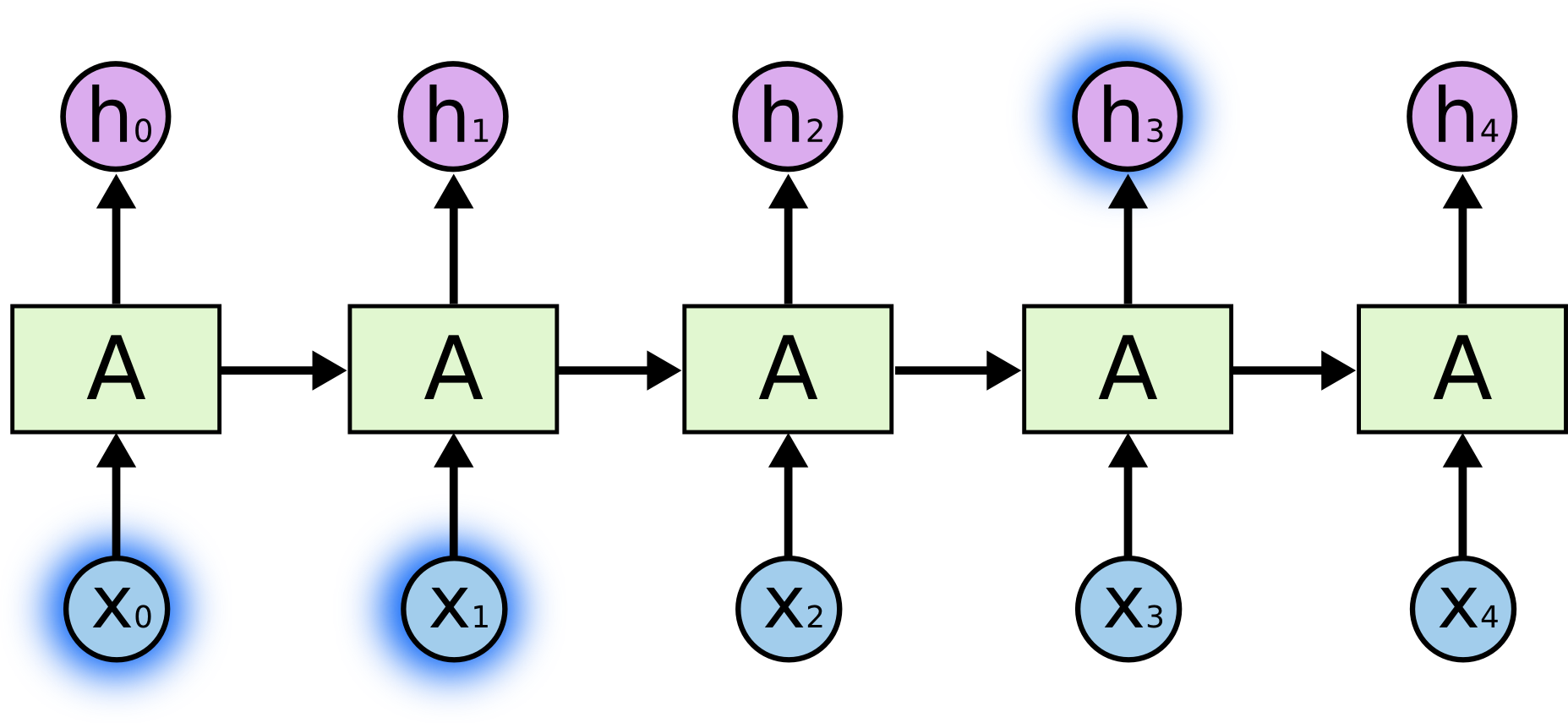
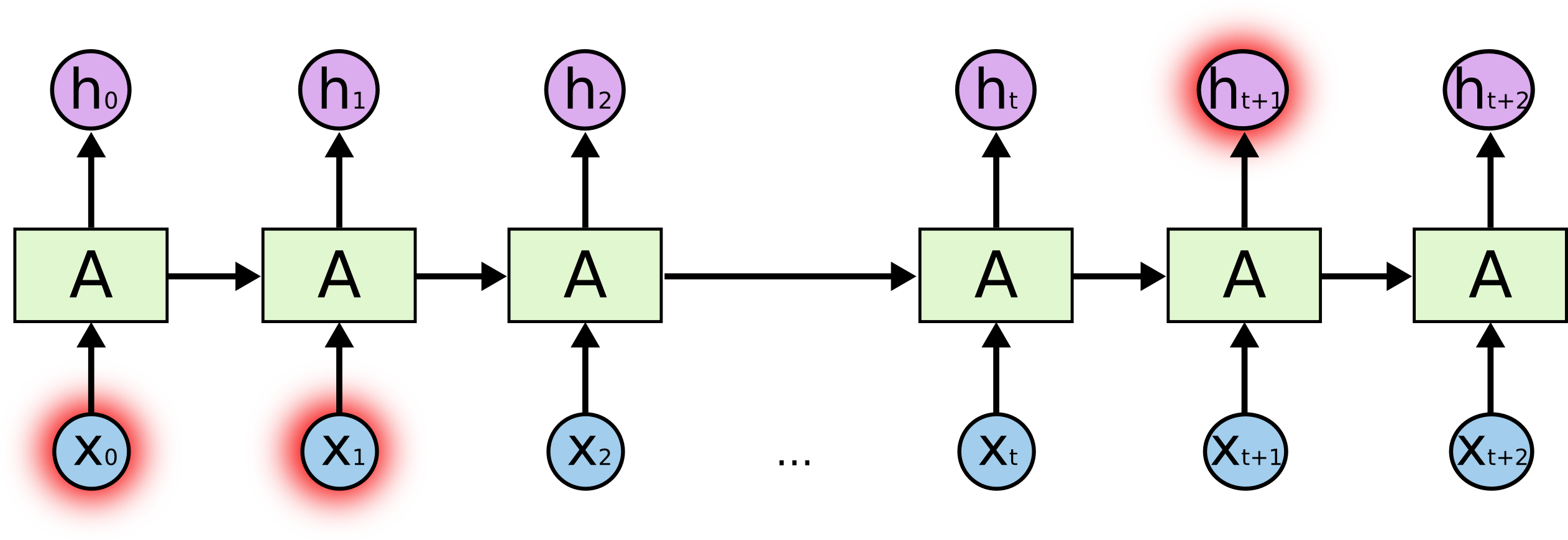
But there are also cases where we need more context. Consider trying to predict the last word in the text “I grew up in France… I speak fluent _French_.” Recent information suggests that the next word is probably the name of a language, but if we want to narrow down which language, we need the context of France, from further back. It’s entirely possible for the gap between the relevant information and the point where it is needed to become very large.
但在某些情况下,我们需要更多的背景信息。考虑试图预测文本“I grew up in France… I speak fluent French.”中的最后一个单词。最近的信息表明下一个单词可能是某种语言的名称,但如果我们想缩小语言范围,我们需要更早的法国这一背景信息。相关信息和需要使用该信息的点之间的间隔完全有可能变得非常大。
Unfortunately, as that gap grows, RNNs become unable to learn to connect the information.
不幸的是,随着这种间隔的扩大,RNN变得无法学习去连接信息。
In theory, RNNs are absolutely capable of handling such “long-term dependencies.” A human could carefully pick parameters for them to solve toy problems of this form. Sadly, in practice, RNNs don’t seem to be able to learn them. The problem was explored in depth by Hochreiter (1991) [German] and Bengio, et al. (1994), who found some pretty fundamental reasons why it might be difficult.
理论上,RNNs完全有能力处理这种“长期依赖”。人类可以仔细挑选参数,使它们解决这种形式的玩具问题。遗憾的是,在实际应用中,RNNs似乎无法学会它们。这个问题在Hochreiter(1991)和Bengio等人(1994)的研究中得到了深入探讨,他们发现了一些可能导致这一困难的基本原因。
Thankfully, LSTMs don’t have this problem!
值得庆幸的是,LSTM 没有这个问题!
LSTM Networks
Long Short Term Memory networks – usually just called “LSTMs” – are a special kind of RNN, capable of learning long-term dependencies. They were introduced by Hochreiter & Schmidhuber (1997), and were refined and popularized by many people in following work.1 They work tremendously well on a large variety of problems, and are now widely used.
长短期记忆网络——通常简称为“LSTMs”——是一种特殊的RNN,能够学习长期依赖。它们由Hochreiter和Schmidhuber(1997)引入,并在随后的工作中被许多人改进和推广。LSTMs在大量不同的问题上表现出色,现在被广泛使用。
LSTMs are explicitly designed to avoid the long-term dependency problem. Remembering information for long periods of time is practically their default behavior, not something they struggle to learn!
LSTMs被明确设计用于避免长期依赖问题。记住长时间的信息几乎是它们的默认行为,而不是它们需要努力学习的东西!
All recurrent neural networks have the form of a chain of repeating modules of neural network. In standard RNNs, this repeating module will have a very simple structure, such as a single tanh layer.
所有递归神经网络都具有神经网络重复模块链的形式。在标准 RNN 中,该重复模块将具有非常简单的结构,例如单个 tanh 层。
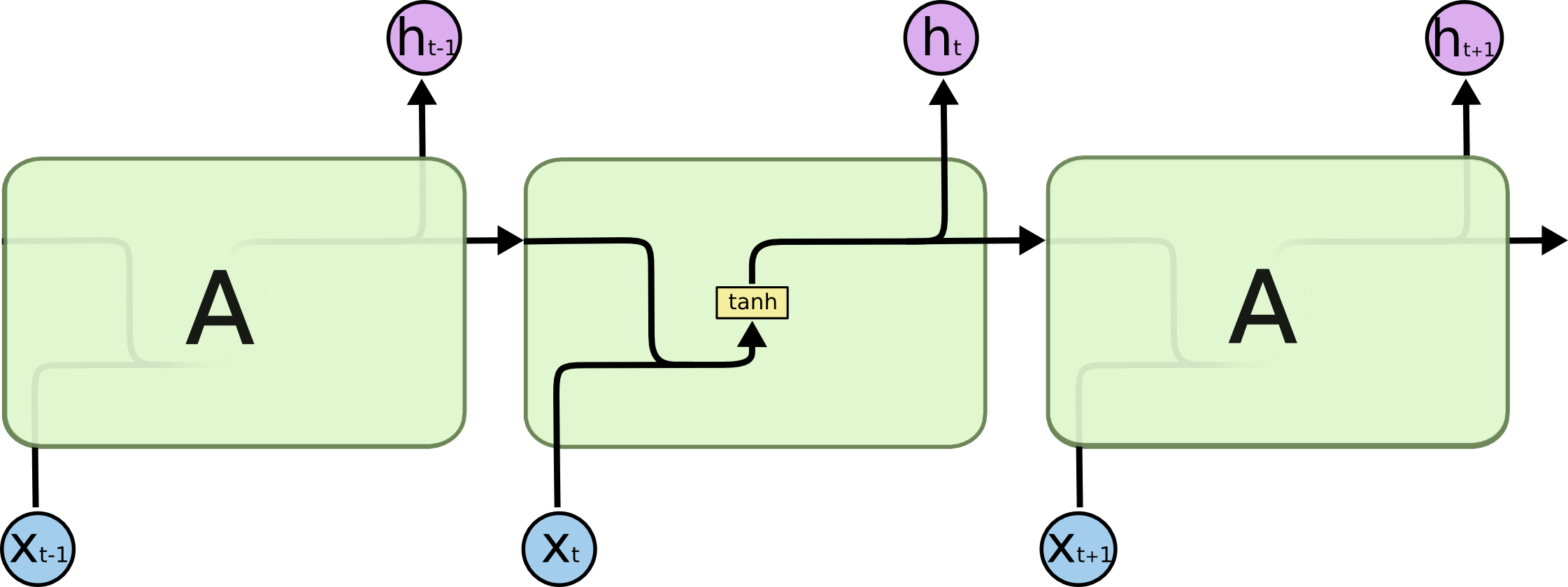
The repeating module in a standard RNN contains a single layer.
标准 RNN 中的重复模块包含单层。
LSTMs also have this chain like structure, but the repeating module has a different structure. Instead of having a single neural network layer, there are four, interacting in a very special way.
LSTM 也具有这种链状结构,但重复模块具有不同的结构。不是只有一个神经网络层,而是有四个,以一种非常特殊的方式进行交互。
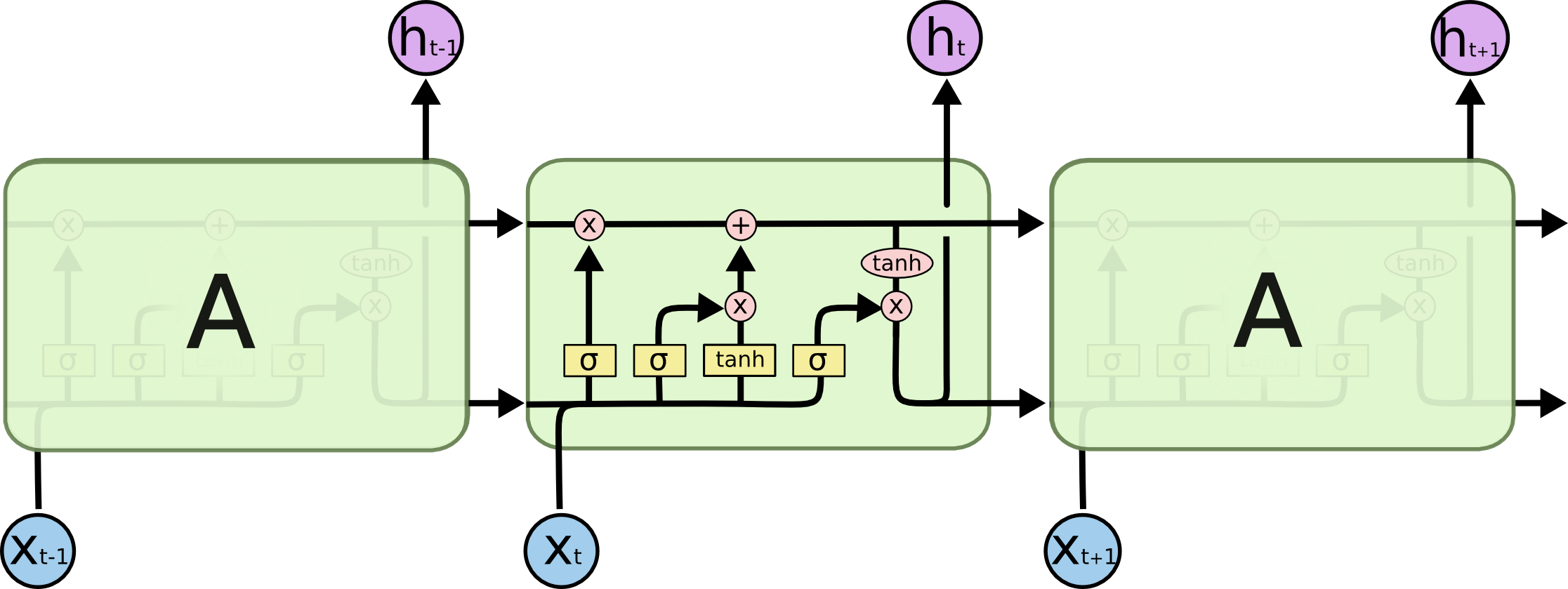
The repeating module in an LSTM contains four interacting layers.
LSTM 中的重复模块包含四个交互层。
Don’t worry about the details of what’s going on. We’ll walk through the LSTM diagram step by step later. For now, let’s just try to get comfortable with the notation we’ll be using.
不用担心具体的细节。我们稍后会一步步讲解LSTM的图表。现在,让我们先熟悉一下我们将要使用的符号。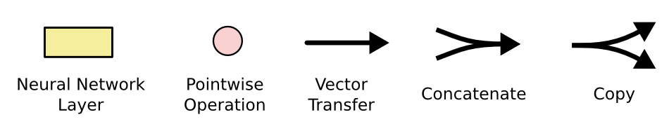
In the above diagram, each line carries an entire vector, from the output of one node to the inputs of others. The pink circles represent pointwise operations, like vector addition, while the yellow boxes are learned neural network layers. Lines merging denote concatenation, while a line forking denote its content being copied and the copies going to different locations.
在上图中,每条线都带有一个完整的向量,从一个节点的输出到其他节点的输入。粉红色的圆圈代表逐点运算,如向量加法,而黄色框是学习的神经网络层。合并的行表示串联,而分叉的行表示正在复制其内容并将副本发送到不同的位置。
The Core Idea Behind LSTMs
LSTM 背后的核心思想
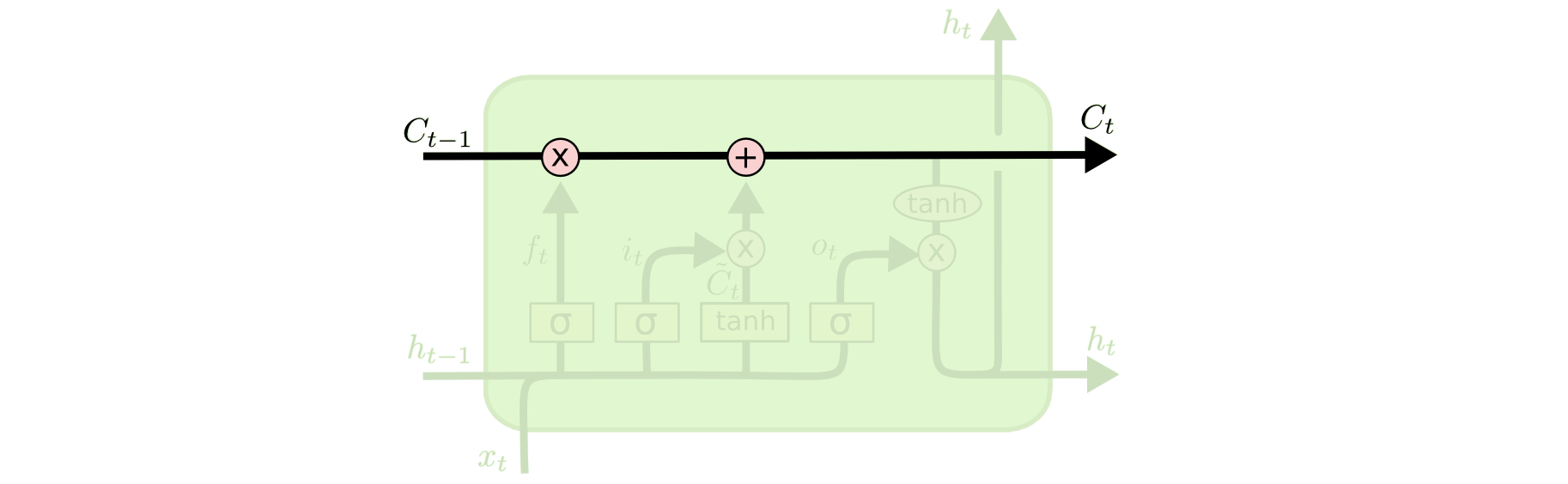
The key to LSTMs is the cell state, the horizontal line running through the top of the diagram.
LSTMs的关键是单元状态,这条横线贯穿了图表的顶部。
The cell state is kind of like a conveyor belt. It runs straight down the entire chain, with only some minor linear interactions. It’s very easy for information to just flow along it unchanged.
单元状态有点像传送带。它直接沿着整个链条运行,只有一些小的线性交互。信息可以非常容易地沿着它不变地流动。
The LSTM does have the ability to remove or add information to the cell state, carefully regulated by structures called gates.
LSTM确实具有从单元状态中移除或添加信息的能力,这些操作由称为门控的结构严格调控。
Gates are a way to optionally let information through. They are composed out of a sigmoid neural net layer and a pointwise multiplication operation.
门控是一种选择性地让信息通过的方式。它们由一个sigmoid神经网络层和一个逐点乘法操作组成。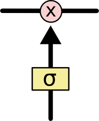
The sigmoid layer outputs numbers between zero and one, describing how much of each component should be let through. A value of zero means “let nothing through,” while a value of one means “let everything through!”
sigmoid 层输出介于 0 和 1 之间的数字,描述每个组件应通过多少。值为零表示“什么都不让通过”,而值为 1 表示“让所有东西都通过!”
An LSTM has three of these gates, to protect and control the cell state.
LSTM 有三个这样的门,用于保护和控制单元状态。
Step-by-Step LSTM Walk Through
循序渐进的 LSTM 演练
forget gate layer
The first step in our LSTM is to decide what information we’re going to throw away from the cell state. This decision is made by a sigmoid layer called the “forget gate layer.” It looks at $h_{t−1}$ and $x_t$, and outputs a number between 00 and 11 for each number in the cell state $C_{t−1}$. A 1 represents “completely keep this” while a 0 represents “completely get rid of this.”
LSTM的第一步是决定要从单元状态中丢弃哪些信息。这个决策是由一个名为“遗忘门层”的sigmoid层做出的。它查看 $h_{t-1}$ 和 $x_t$,并为单元状态 $C_{t-1}$ 中的每个数字输出一个介于0和1之间的数值。1表示“完全保留这个”,而0表示“完全丢弃这个”。
Let’s go back to our example of a language model trying to predict the next word based on all the previous ones. In such a problem, the cell state might include the gender of the present subject, so that the correct pronouns can be used. When we see a new subject, we want to forget the gender of the old subject.
让我们回到我们的例子,一个语言模型试图基于所有前面的单词来预测下一个单词。在这样的问题中,单元状态可能包含当前主语的性别,以便使用正确的代词。当我们看到一个新的主语时,我们想忘记旧主语的性别。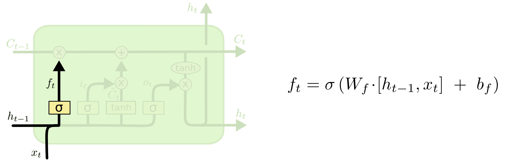
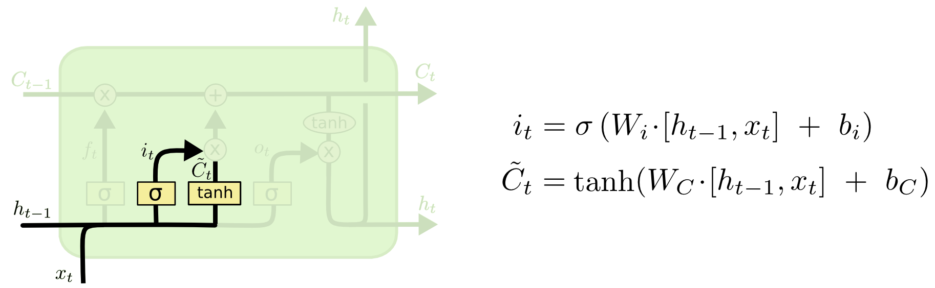
input gate layer
The next step is to decide what new information we’re going to store in the cell state. This has two parts. First, a sigmoid layer called the “input gate layer” decides which values we’ll update. Next, a tanh layer creates a vector of new candidate values, $\tilde{C}_t$, that could be added to the state. In the next step, we’ll combine these two to create an update to the state.
下一步是决定要在单元状态中存储哪些新信息。这包括两个部分。首先,一个名为“输入门层”的sigmoid层决定我们将更新哪些值。接下来,一个tanh层创建一个新的候选值向量$\tilde{C}_t$,这些候选值可以被添加到状态中。在下一步中,我们将结合这两部分来更新状态。
In the example of our language model, we’d want to add the gender of the new subject to the cell state, to replace the old one we’re forgetting.
在我们的语言模型示例中,我们希望将新主语的性别添加到单元格状态中,以替换我们忘记的旧主语。
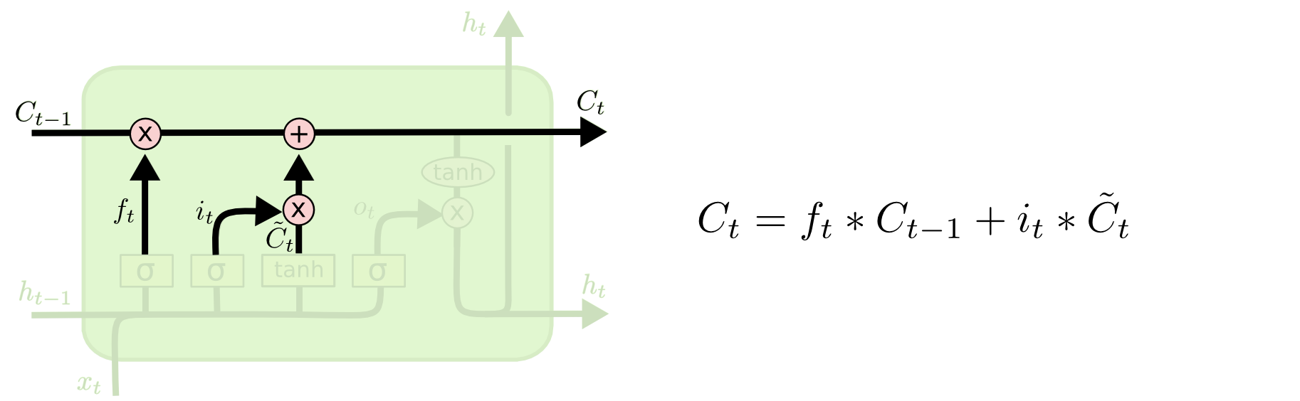
It’s now time to update the old cell state$C_{t-1}$, into the new cell state $C_t$. The previous steps already decided what to do, we just need to actually do it.
现在是时候将旧的单元格状态$C_{t-1}$更新为新的单元格状态 $C_t$了。前面的步骤已经决定了要做什么,我们只需要实际去执行它。
We multiply the old state by $𝑓_𝑡$, forgetting the things we decided to forget earlier. Then we add $i_t \ast \tilde{C}_t$. This is the new candidate values, scaled by how much we decided to update each state value.
我们将旧状态乘以 $f_t$,忘记我们之前决定忘记的内容。然后我们加上 $i_t \ast \tilde{C}_t$。这些是新的候选值,按我们决定更新每个状态值的程度进行缩放。
In the case of the language model, this is where we’d actually drop the information about the old subject’s gender and add the new information, as we decided in the previous steps.
在语言模型的情况下,正如我们在前面的步骤中决定的那样,我们实际上会删除有关旧主题性别的信息并添加新信息。
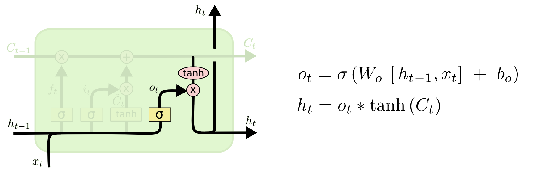
output layer
Finally, we need to decide what we’re going to output. This output will be based on our cell state, but will be a filtered version. First, we run a sigmoid layer which decides what parts of the cell state we’re going to output. Then, we put the cell state through tanh (to push the values to be between −1 and 1) and multiply it by the output of the sigmoid gate, so that we only output the parts we decided to.
最后,我们需要决定输出什么。这个输出将基于我们的单元状态,但会是一个过滤后的版本。首先,我们运行一个sigmoid层来决定要输出单元状态的哪些部分。然后,我们将单元状态通过tanh(将值压缩到-1到1之间),并将其与sigmoid门的输出相乘,这样我们只输出我们决定输出的部分。
For the language model example, since it just saw a subject, it might want to output information relevant to a verb, in case that’s what is coming next. For example, it might output whether the subject is singular or plural, so that we know what form a verb should be conjugated into if that’s what follows next.
对于语言模型的例子,由于它刚刚看到一个主语,它可能想输出与动词相关的信息,以防接下来需要动词。例如,它可能会输出主语是单数还是复数,这样我们就知道如果接下来是动词,该动词应该变成什么形式。
Variants on Long Short Term Memory
长短期记忆的变体
What I’ve described so far is a pretty normal LSTM. But not all LSTMs are the same as the above. In fact, it seems like almost every paper involving LSTMs uses a slightly different version. The differences are minor, but it’s worth mentioning some of them.
我到目前为止描述的是一个相当普通的LSTM。但并不是所有的LSTM都与上述相同。实际上,几乎每篇涉及LSTM的论文都使用了稍微不同的版本。这些差异很小,但值得一提。
One popular LSTM variant, introduced by Gers & Schmidhuber (2000), is adding “peephole connections.” This means that we let the gate layers look at the cell state.
一个由Gers和Schmidhuber(2000)引入的流行LSTM变体是添加“窥视连接”。这意味着我们让门控层查看单元状态。
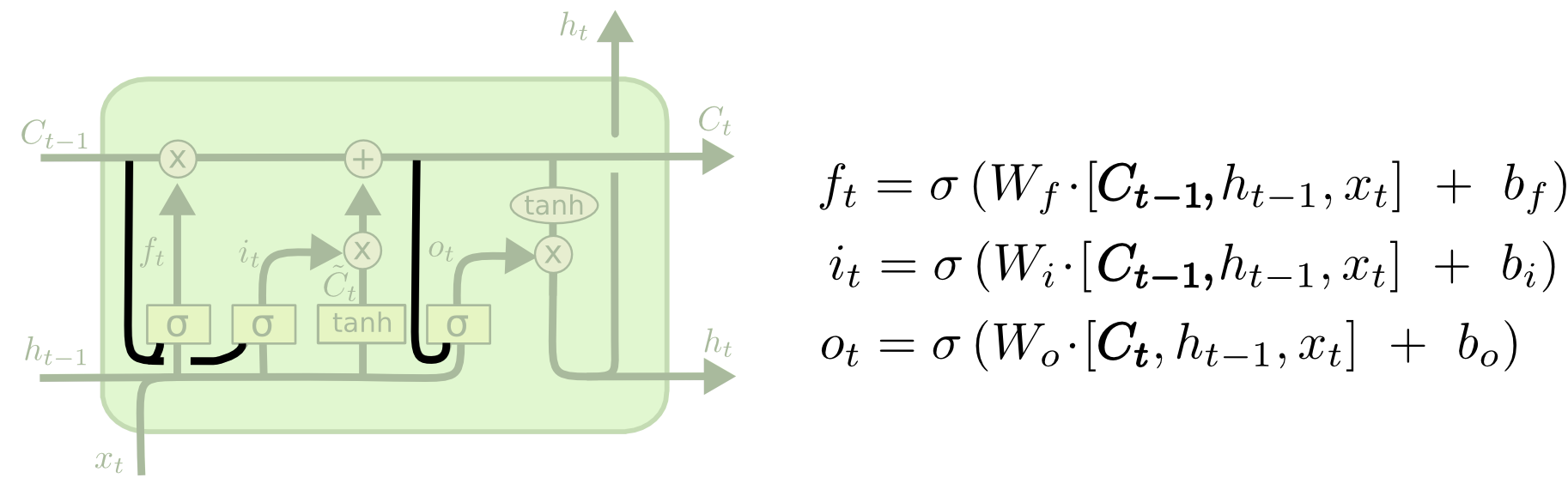
The above diagram adds peepholes to all the gates, but many papers will give some peepholes and not others.
上图为所有门控添加了窥视连接,但许多论文会只为部分门控添加窥视连接,而不是全部。
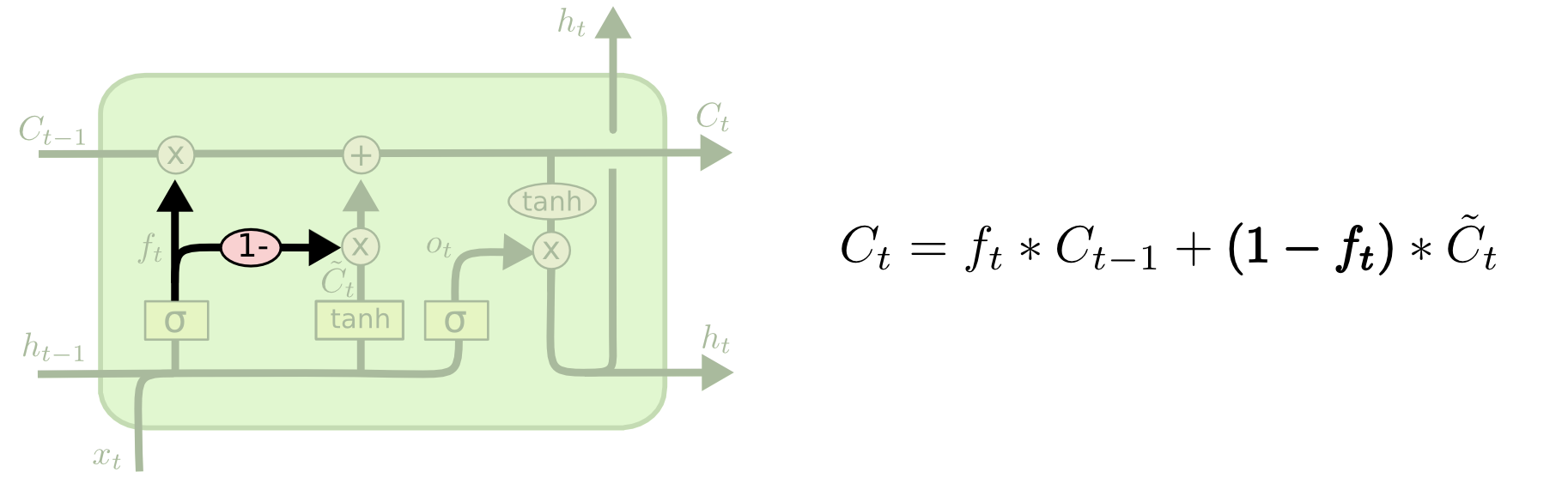
Another variation is to use coupled forget and input gates. Instead of separately deciding what to forget and what we should add new information to, we make those decisions together. We only forget when we’re going to input something in its place. We only input new values to the state when we forget something older.
另一种变体是使用耦合的遗忘门和输入门。我们不是分别决定要忘记什么以及要添加什么新信息,而是将这些决策结合在一起。我们只有在要输入新信息时才会忘记某些内容。只有在忘记旧信息时,我们才会将新值输入到状态中。
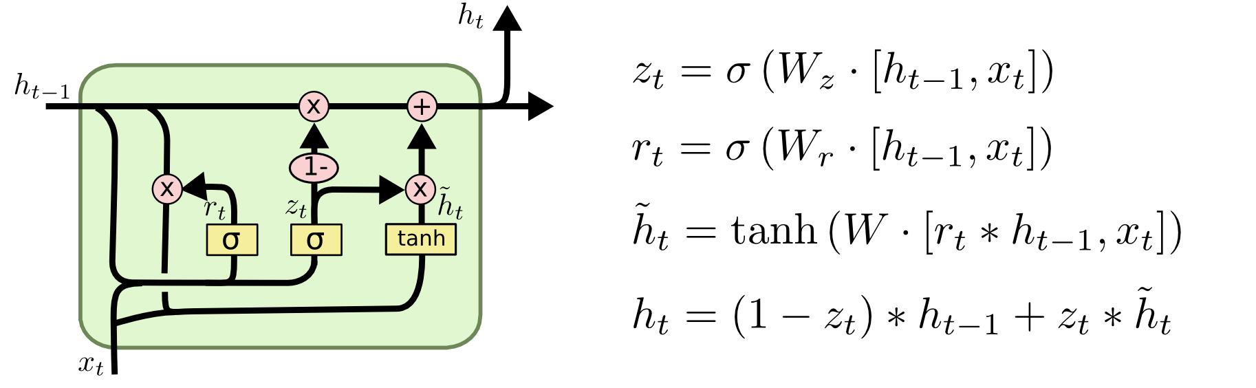
A slightly more dramatic variation on the LSTM is the Gated Recurrent Unit, or GRU, introduced by Cho, et al. (2014). It combines the forget and input gates into a single “update gate.” It also merges the cell state and hidden state, and makes some other changes. The resulting model is simpler than standard LSTM models, and has been growing increasingly popular.
LSTM的一个稍微更显著的变体是门控循环单元(GRU),由Cho等人(2014)引入。它将遗忘门和输入门组合成一个“更新门”。它还合并了单元状态和隐藏状态,并做了一些其他的改变。最终的模型比标准的LSTM模型更简单,并且越来越受欢迎。
These are only a few of the most notable LSTM variants. There are lots of others, like Depth Gated RNNs by Yao, et al. (2015). There’s also some completely different approach to tackling long-term dependencies, like Clockwork RNNs by Koutnik, et al. (2014).
这些只是一些最著名的LSTM变体。还有许多其他变体,例如Yao等人(2015)提出的深度门控RNN。此外,还有一些完全不同的方法来解决长期依赖问题,例如Koutnik等人(2014)提出的时钟式RNN。
Which of these variants is best? Do the differences matter? Greff, et al. (2015) do a nice comparison of popular variants, finding that they’re all about the same. Jozefowicz, et al. (2015) tested more than ten thousand RNN architectures, finding some that worked better than LSTMs on certain tasks.
这些变体中哪一个最好?差异重要吗?Greff等人(2015)对流行变体进行了很好的比较,发现它们的表现几乎相同。Jozefowicz等人(2015)测试了超过一万种RNN架构,发现其中一些在某些任务上的表现比LSTMs更好。
Conclusion 结论
Earlier, I mentioned the remarkable results people are achieving with RNNs. Essentially all of these are achieved using LSTMs. They really work a lot better for most tasks!
前面,我提到了人们用递归神经网络(RNNs)取得的显著成果。基本上所有这些成果都是使用LSTMs实现的。对于大多数任务,LSTMs的效果确实要好得多!
Written down as a set of equations, LSTMs look pretty intimidating. Hopefully, walking through them step by step in this essay has made them a bit more approachable.
作为一组方程写下来,LSTMs看起来相当令人生畏。希望通过在本文中一步一步地讲解它们,使它们变得更容易理解。
LSTMs were a big step in what we can accomplish with RNNs. It’s natural to wonder: is there another big step? A common opinion among researchers is: “Yes! There is a next step and it’s attention!” The idea is to let every step of an RNN pick information to look at from some larger collection of information. For example, if you are using an RNN to create a caption describing an image, it might pick a part of the image to look at for every word it outputs. In fact, Xu, _et al._ (2015) do exactly this – it might be a fun starting point if you want to explore attention! There’s been a number of really exciting results using attention, and it seems like a lot more are around the corner…
LSTMs是我们用RNNs能实现的一个大进步。很自然地会有人问:还有另一个大进步吗?研究人员的一个普遍看法是:“是的!下一个进步是注意力机制!”这个想法是让RNN的每一步都从一些更大的信息集合中选择要看的信息。例如,如果你使用RNN来创建描述图像的标题,它可能会为它输出的每个单词选择图像的一部分。事实上,Xu等人(2015)正是这样做的——如果你想探索注意力机制,这可能是一个有趣的起点!使用注意力机制已经取得了许多非常令人兴奋的成果,似乎还会有更多的成果即将到来……
Attention isn’t the only exciting thread in RNN research. For example, Grid LSTMs by Kalchbrenner, _et al._ (2015) seem extremely promising. Work using RNNs in generative models – such as Gregor, _et al._ (2015), Chung, _et al._ (2015), or Bayer & Osendorfer (2015) – also seems very interesting. The last few years have been an exciting time for recurrent neural networks, and the coming ones promise to only be more so!
注意力机制并不是RNN研究中唯一令人兴奋的方向。例如,Kalchbrenner等人(2015)的Grid LSTMs看起来非常有前途。在生成模型中使用RNN的工作——例如Gregor等人(2015)、Chung等人(2015)或Bayer和Osendorfer(2015)的工作——也非常有趣。过去几年是递归神经网络的激动人心的时期,未来几年只会更加激动人心!
Acknowledgments 确认
I’m grateful to a number of people for helping me better understand LSTMs, commenting on the visualizations, and providing feedback on this post.
我感谢许多人帮助我更好地理解 LSTM,对可视化进行评论,并对这篇文章提供反馈。
I’m very grateful to my colleagues at Google for their helpful feedback, especially Oriol Vinyals, Greg Corrado, Jon Shlens, Luke Vilnis, and Ilya Sutskever. I’m also thankful to many other friends and colleagues for taking the time to help me, including Dario Amodei, and Jacob Steinhardt. I’m especially thankful to Kyunghyun Cho for extremely thoughtful correspondence about my diagrams.
我非常感谢 Google 同事提供的有益反馈,尤其是 Oriol Vinyals、Greg Corrado、Jon Shlens、Luke Villnis 和 Ilya Sutskever。我还要感谢许多其他朋友和同事抽出时间帮助我,包括 Dario Amodei 和 Jacob Steinhardt。我特别感谢 Kyunghyun Cho 对我的图表进行了非常周到的通信。
Before this post, I practiced explaining LSTMs during two seminar series I taught on neural networks. Thanks to everyone who participated in those for their patience with me, and for their feedback.
在这篇文章之前,我在我教授的关于神经网络的两个系列研讨会上练习了解释 LSTM。感谢所有参与活动的人对我的耐心和反馈。
注释-如何理解门控结构的计算
根据前面的文章, 我们已经知道基础 神经网络和 基础RNN 中,数据从输入层到隐藏层到输出层的计算,这里再复习一下
基础神经网络
隐藏层
$h_t=f(W_{xh}x_t+b_h)$
- $x_t$:当前输入
- $W_{xh}$:输入层到隐藏层的权重矩阵
- $b_h$:偏置
- $f$:激活函数(如tanh或ReLU)
计算隐藏状态分为2个步骤
RNN的隐藏层具有循环连接,即多了一个隐藏层到隐藏层的权重矩阵参与计算 ,使得每个隐藏状态依赖于前一时间步的隐藏状态和当前时间步的输入。公式如下:
$h_t=f(W_{hh}h_{t−1}+W_{xh}x_t+b_h)$
- $h_t$:当前时间步的隐藏状态
- $h_{t-1}$:前一时间步的隐藏状态
- $x_t$:当前时间步的输入
- $W_{hh}$:隐藏状态到隐藏状态的权重矩阵
- $W_{xh}$:输入到隐藏状态的权重矩阵
- $b_h$:偏置
- $f$:激活函数(如tanh或ReLU)
从上面文章中可以看到, 不论计算过程在复杂,都是要根据输入求输出。。 而在LSTM 中, 复杂的点在于。隐藏层的计算由简单的隐藏层-隐藏层权重矩阵参与计算 拆分成了多个步骤
LSTM
1. 遗忘门(Forget Gate)
遗忘门控制单元状态中哪些信息需要被保留或丢弃。遗忘门接收当前时间步的输入 $x_t$和前一时间步的隐藏状态 $h_{t-1}$,通过一个$Sigmoid$函数计算得到一个介于0和1之间的标量(或向量),用于缩放前一时间步的细胞状态。
公式如下: $f_t = \sigma(W_f \cdot [h_{t-1}, x_t] + b_f)$
如果把层级关系也在公式中体现出来,该公式可以细化成如下格式:
$f_t^l = \sigma(W_f \cdot [h_{t-1}^l, x_t^{l-1}] + b_f)$
其中 $x$ 也可以替换成其他变量,只要是代表当前时间步的输入即可。
例如在 RECURRENT NEURAL NETWORK REGULARIZATION 该公式就表示成了 $f_t^l = \sigma(W_f \cdot [h_{t-1}^l, h_t^{l-1}] + b_f)$
- $[h_t, x_{t-1}]$或者$[h_t^{l-1}, h_{t-1}^l]$表示将当前输入和前一时间步的隐藏状态向量拼接成一个向量。
- $W_f$ 是该遗忘门的权重矩阵。
- $b_f$ 是偏置向量。
- $\sigma$ 是$sigmoid$ 非线性激活函数,输出范围在0到1之间。
2. 输入门(Input Gate)
输入门控制新信息写入单元状态的过程。输入门同样接收当前时间步的输入 $x_t$和前一时间步的隐藏状态 $h_{t-1}$,并通过Sigmoid函数生成一个介于0和1之间的标量,表示允许多少新信息进入细胞状态。0表示完全不允许新信息进入,1表示完全允许新信息进入。
$tanh$层生成候选单元状态。
公式如下:
$i_t = \sigma(W_i \cdot [h_{t-1}, x_t] + b_i)$
$\tilde{C}_t = \tanh(W_C \cdot [h_{t-1}, x_t] + b_C)$
$W_i$:输入门的权重矩阵,用于将前一时间步的隐藏状态和当前时间步的输入进行线性变换。
$W_C$:候选细胞状态的权重矩阵,用于将前一时间步的隐藏状态和当前时间步的输入进行线性变换。
3. 单元状态(Cell State)
单元状态 $C_t$ 是LSTM单元内部的长期记忆,它在时间步之间几乎直接传递,通过遗忘门和输入门的调节进行更新。新的单元状态由前一时间步的单元状态乘以遗忘门的输出加上输入门输出和候选值的乘积得到。
公式如下:$C_t = f_t \cdot C_{t-1} + i_t \cdot \tilde{C}_t$
4. 输出门(Output Gate)- 得到隐藏状态
输出门决定哪些信息从细胞状态传递到隐藏状态(LSTM单元的输出)。输出门通过Sigmoid函数决定哪些信息将被输出,并将细胞状态通过Tanh层处理后乘以该输出。
公式如下:
$o_t = \sigma(W_o \cdot [h_{t-1}, x_t] + b_o)$
$h_t = o_t \cdot \tanh(C_t)$