RECURRENT NEURAL NETWORK REGULARIZATION

ABSTRACT 摘要

We present a simple regularization technique for Recurrent Neural Networks (RNNs) with Long Short-Term Memory (LSTM) units. Dropout, the most suc- cessful technique for regularizing neural networks, does not work well with RNNs and LSTMs. In this paper, we show how to correctly apply dropout to LSTMs, and show that it substantially reduces overfitting on a variety of tasks. These tasks include language modeling, speech recognition, image caption generation, and machine translation.
我们提出了一种用于长短期记忆（LSTM）单元的循环神经网络（RNN）的简单正则化技术。最成功的正则化神经网络技术——Dropout，在RNN和LSTM上效果不好。在本文中，我们展示了如何正确地将Dropout应用于LSTM，并证明它在各种任务上显著减少了过拟合。这些任务包括语言建模、语音识别、图像描述生成和机器翻译。

1 INTRODUCTION 引言

The Recurrent Neural Network (RNN) is neural sequence model that achieves state of the art per- formance on important tasks that include language modeling Mikolov (2012), speech recognition Graves et al. (2013), and machine translation Kalchbrenner & Blunsom (2013). It is known that successful applications of neural networks require good regularization. Unfortunately, dropout Srivastava (2013), the most powerful regularization method for feedforward neural networks, does not work well with RNNs. As a result, practical applications of RNNs often use models that are too small because large RNNs tend to overfit. Existing regularization methods give relatively small improvements for RNNs Graves (2013). In this work, we show that dropout, when correctly used, greatly reduces overfitting in LSTMs, and evaluate it on three different problems.

The code for this work can be found in https://github.com/wojzaremba/lstm.

递归神经网络（RNN）是一种神经序列模型，可在重要任务上实现最先进的性能，包括语言建模Mikolov（2012），语音识别Graves等人（2013）和机器翻译Kalchbrenner&Blunsom（2013）。众所周知，神经网络的成功应用需要良好的正则化。不幸的是，dropout Srivastava （2013） 是前馈神经网络最强大的正则化方法，但不能很好地用于 RNN。因此，RNN 的实际应用通常使用太小的模型，因为大型 RNN 往往会过度拟合。现有的正则化方法对RNNs Graves（2013）进行了相对较小的改进。在这项工作中，我们表明，如果正确使用，压差可以大大减少LSTM中的过拟合，并在三个不同的问题上对其进行评估。

此工作的代码可以在https://github.com/wojzaremba/lstm找到。

2 RELATED WORK

Dropout Srivastava (2013) is a recently introduced regularization method that has been very suc- cessful with feed-forward neural networks. While much work has extended dropout in various ways Wang & Manning (2013); Wan et al. (2013), there has been relatively little research in applying it to RNNs. The only paper on this topic is by Bayer et al. (2013), who focuses on “marginalized dropout” Wang & Manning (2013), a noiseless deterministic approximation to standard dropout. Bayer et al. (2013) claim that conventional dropout does not work well with RNNs because the re- currence amplifies noise, which in turn hurts learning. In this work, we show that this problem can be fixed by applying dropout to a certain subset of the RNNs’ connections. As a result, RNNs can now also benefit from dropout.
Dropout Srivastava（2013）是一种最近引入的正则化方法，在前馈神经网络中非常成功。尽管很多工作以各种方式扩展了Dropout Wang & Manning（2013）；Wan等（2013），但在RNN上应用它的研究相对较少。关于这个主题的唯一论文是Bayer等人（2013）的，他们专注于“边缘化Dropout” Wang & Manning（2013），这是标准Dropout的一种无噪声确定性近似。Bayer等人（2013）认为传统的Dropout在RNN上效果不好，因为递归放大了噪声，进而影响了学习。在这项工作中，我们展示了通过将Dropout应用于RNN连接的某个子集可以解决这个问题。因此，RNN现在也可以受益于Dropout。

Independently of our work, Pham et al. (2013) developed the very same RNN regularization method and applied it to handwriting recognition. We rediscovered this method and demonstrated strong empirical results over a wide range of problems. Other work that applied dropout to LSTMs is Pachitariu & Sahani (2013).
独立于我们的工作，Pham等人（2013）开发了完全相同的RNN正则化方法并将其应用于手写识别。我们重新发现了这种方法，并在广泛的问题上展示了强大的实证结果。其他将Dropout应用于LSTM的工作包括Pachitariu & Sahani（2013）。

There have been a number of architectural variants of the RNN that perform better on problems with long term dependencies Hochreiter & Schmidhuber (1997); Graves et al. (2009); Cho et al. (2014); Jaeger et al. (2007); Koutník et al. (2014); Sundermeyer et al. (2012). In this work, we show how to correctly apply dropout to LSTMs, the most commonly-used RNN variant; this way of applying dropout is likely to work well with other RNN architectures as well. In this paper, we consider the following tasks: language modeling, speech recognition, and machine translation. Language modeling is the first task where RNNs have achieved substantial success Mikolov et al. (2010; 2011); Pascanu et al. (2013). RNNs have also been successfully used for speech recognition Robinson et al. (1996); Graves et al. (2013) and have recently been applied to machine translation, where they are used for language modeling, re-ranking, or phrase modeling Devlin et al. (2014); Kalchbrenner & Blunsom (2013); Cho et al. (2014); Chow et al. (1987); Mikolov et al. (2013).
已经有许多RNN的架构变体在处理长期依赖问题上表现更好： Hochreiter & Schmidhuber (1997); Graves等（2009）；Cho等（2014）；Jaeger等（2007）；Koutník等（2014）；Sundermeyer等（2012）。在这项工作中，我们展示了如何正确地将dropout应用于LSTM，这是最常用的RNN变体；这种应用dropout的方法也可能适用于其他RNN架构。在本文中，我们考虑了以下任务：语言建模、语音识别和机器翻译。语言建模是RNN首次取得显著成功的任务 Mikolov等（2010；2011）；Pascanu等（2013）。RNN也已成功应用于语音识别 Robinson等（1996）；Graves等（2013），并且最近被应用于机器翻译，在那里它们被用于语言建模、重排序或短语建模 Devlin等（2014）；Kalchbrenner & Blunsom（2013）；Cho等（2014）；Chow等（1987）；Mikolov等（2013）。

3 REGULARIZING RNNS WITH LSTM CELLS 使用LSTM单元对RNN进行正则化

In this section we describe the deep LSTM (Section 3.1). Next, we show how to regularize them (Section 3.2), and explain why our regularization scheme works.
在本节中，我们描述了深度LSTM（3.1节）。接下来，我们展示如何对它们进行正则化（3.2节），并解释我们的正则化方案为何有效。

We let subscripts denote timesteps and superscripts denote layers. All our states are n-dimensional. Let $h_t^l \in \mathbb{R}^n$ be a hidden state in layer$l$ in timestep $t$. Moreover, let $T_{n,m} : \mathbb{R}^n \to \mathbb{R}^m$be an affine transform ($Wx + b$ for some $W$ and $b$). Let $\odot$ be element-wise multiplication and let $h_t^0​$ be an input word vector at timestep $k$. We use the activations $h_t^L$​ to predict $y_t$​, since $L$ is the number of layers in our deep LSTM.
我们用下标表示时间步长，用上标表示层次。我们所有的状态都是n维的。令$h_t^l \in \mathbb{R}^n$ 为时间步$t$中层$l$的隐藏状态。此外，令$T_{n,m} : \mathbb{R}^n \to \mathbb{R}^m$为仿射变换（某些$W$和$b$,$Wx + b$）。令$\odot$为逐元素乘法，并令$h_t^0$​为时间步$k$的输入词向量。我们使用激活值$h_t^L$​来预测$y_t​$，因为$L$是我们深度LSTM的层数。

3.1 LONG-SHORT TERM MEMORY UNITS 长短期记忆单元

The RNN dynamics can be described using deterministic transitions from previous to current hidden states. The deterministic state transition is a function
RNN的动态可以用从先前隐藏状态到当前隐藏状态的确定性转换来描述。确定性状态转换是一个函数

RNN : $h_t^{l-1}​$, $h_{t-1}^l \rightarrow h_t^l$

For classical RNNs, this function is given by
$h_t^l = f(T_{n,n} h_t^{l-1} + T_{n,n} h_{t-1}^l), where f \in \{\text{sigm, tanh}\}$

The LSTM has complicated dynamics that allow it to easily “memorize” information for an extended number of timesteps. The “long term” memory is stored in a vector of memory cells $c_t^l \in \mathbb{R}^n$. Although many LSTM architectures that differ in their connectivity structure and activation functions, all LSTM architectures have explicit memory cells for storing information for long periods of time. The LSTM can decide to overwrite the memory cell, retrieve it, or keep it for the next time step. The LSTM architecture used in our experiments is given by the following equations Graves et al. (2013):
LSTM具有复杂的动态，允许它轻松地“记住”多个时间步长的信息。“长期”记忆存储在记忆单元向量$c_t^l \in \mathbb{R}^n$中。尽管许多LSTM架构在连接结构和激活函数上有所不同，但所有LSTM架构都有明确的记忆单元用于长时间存储信息。LSTM可以决定覆盖记忆单元、检索或者在下一个时间步中保留它。我们实验中使用的LSTM架构由以下方程给出 Graves等（2013）：

LSTM : $h_t^{l-1}$, $h_{t-1}^l$, $c_{t-1}^l \rightarrow h_t^l$​, $c_t^l$

$\left( \begin{array}{c} i \ f \ o \ g \end{array} \right) = \left( \begin{array}{c} \text{sigm} \ \text{sigm} \ \text{sigm} \ \text{tanh} \end{array} \right) T_{2n,4n} \left( \begin{array}{c} h_{t}^{l-1} \ h_{t-1}^{l} \end{array} \right)​$

$c_t^l = f \odot c_{t-1}^l + i \odot g$

$h_t^l = o \odot \text{tanh}(c_t^l)$
In these equations, sigm and tanh are applied element-wise. Figure 1 illustrates the LSTM equations.
在这些方程中，sigm和tanh逐元素应用。图1展示了LSTM方程

3.2 REGULARIZATION WITH DROPOUT

The main contribution of this paper is a recipe for applying dropout to LSTMs in a way that success-fully reduces overfitting. The main idea is to apply the dropout operator only to the non-recurrent
本文的主要贡献是提供了一种将dropout应用于LSTM的方法，从而成功地减少了过拟合。主要思想是仅将dropout操作符应用于非递归连接。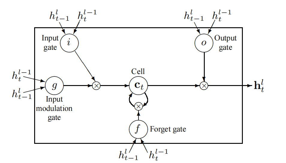

Figure 1: A graphical representation of LSTM memory cells used in this paper (there are minor differences in comparison to Graves (2013)).
图1：本文中使用的LSTM记忆单元的图形表示（与Graves（2013）相比有细微差别）。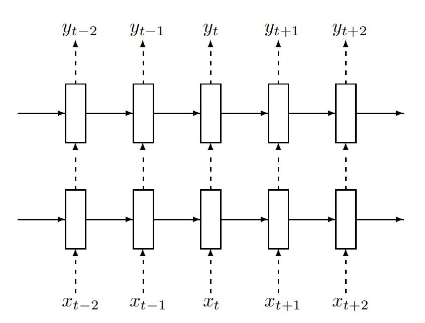

Figure 2: Regularized multilayer RNN. The dashed arrows indicate connections where dropout is applied, and the solid lines indicate connections where dropout is not applied.
图2：正则化的多层RNN。虚线箭头表示应用了dropout的连接，实线表示未应用dropout的连接。
⚠️： x 表示输入层， y 表示输出层

connections (Figure 2). The following equation describes it more precisely, where D is the dropoutoperator that sets a random subset of its argument to zero:
连接（图2）。以下方程更准确地描述了这一点，其中 $D$ 是将其参数的随机子集设置为零的dropout操作符：

$\left( \begin{array}{c} i \ f \ o \ g \end{array} \right) = \left( \begin{array}{c} \text{sigm} \ \text{sigm} \ \text{sigm} \ \text{tanh} \end{array} \right) T_{2n,4n} \left( \begin{array}{c} {D}(h_{t}^{l-1}) \ h_{t-1}^{l} \end{array} \right)​$

$c_t^l = f \odot c_{t-1}^l + i \odot g$

$h_t^l = o \odot \text{tanh}(c_t^l)$

Our method works as follows. The dropout operator corrupts the information carried by the units,forcing them to perform their intermediate computations more robustly. At the same time, we do not want to erase all the information from the units. It is especially important that the units remember
events that occurred many timesteps in the past. Figure 3 shows how information could flow from an event that occurred at timestep t − 2 to the prediction in timestep t + 2 in our implementation of dropout. We can see that the information is corrupted by the dropout operator exactly L + 1 times,
我们的方法如下。dropout 运算符会破坏单元携带的信息，迫使它们更稳健地执行中间计算。同时，我们不想抹去单元的所有信息。特别重要的是，单元需要记住许多时间步长之前发生的事件。图3显示了在我们实现的dropout中，信息如何从时间步 $t-2$ 传递到时间步 $t+2$ 的预测。我们可以看到，信息恰好被dropout操作符破坏了 $L+1$ 次。

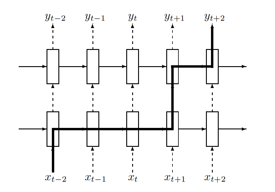
Figure 3: The thick line shows a typical path of information flow in the LSTM. The information is affected by dropout L + 1 times, where L is depth of network.
图 3：粗线显示了 LSTM 中信息流的典型路径。信息受 L + 1 次的dropout影响，其中 L 是网络深度。

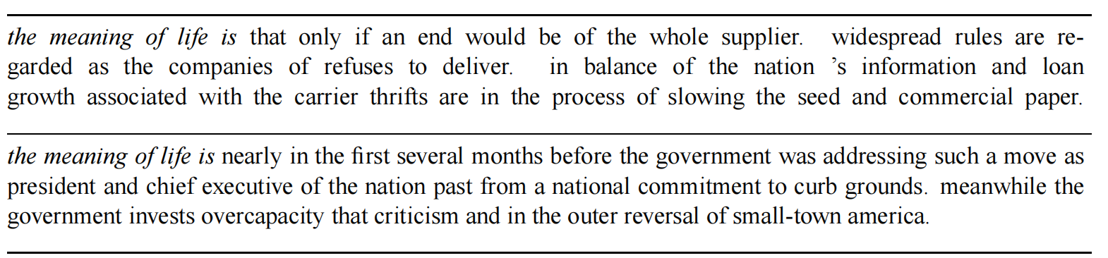
Figure 4: Some interesting samples drawn from a large regularized model conditioned on “The meaning of life is”. We have removed “unk”, “N”, “$” from the set of permissible words.
图4：从一个以“The meaning of life is”为条件的大型正则化模型中抽取的一些有趣样本。我们已经从允许的单词集中移除了“unk”、“N”、“$”。

and this number is independent of the number of timesteps traversed by the information. Standard dropout perturbs the recurrent connections, which makes it difficult for the LSTM to learn to store information for long periods of time. By not using dropout on the recurrent connections, the LSTM can benefit from dropout regularization without sacrificing its valuable memorization ability.
这个数字与信息经过的时间步数无关。标准的dropout会扰乱递归连接，这使得LSTM难以学习长时间存储信息。通过不在递归连接上使用dropout，LSTM可以从dropout正则化中受益，而不牺牲其宝贵的记忆能力。

4 EXPERIMENTS 实验

We present results in three domains: language modeling (Section 4.1), speech recognition (Section 4.2), machine translation (Section 4.3), and image caption generation (Section 4.4).
我们在三个领域中展示了结果：语言建模（第4.1节）、语音识别（第4.2节）、机器翻译（第4.3节）和图像描述生成（第4.4节）。

4.1 LANGUAGE MODELING 语言建模

We conducted word-level prediction experiments on the Penn Tree Bank (PTB) dataset Marcus et al. (1993), which consists of 929k training words, 73k validation words, and 82k test words. It has 10k words in its vocabulary. We downloaded it from Tomas Mikolov’s webpage†. We trained regularized LSTMs of two sizes; these are denoted the medium LSTM and large LSTM. Both LSTMs have two layers and are unrolled for 35 steps. We initialize the hidden states to zero. We then use the final hidden states of the current minibatch as the initial hidden state of the subsequent minibatch (successive minibatches sequentially traverse the training set). The size of each minibatch is 20.
我们在Penn Tree Bank (PTB)数据集上进行了词级预测实验，该数据集包括92.9万个训练词、7.3万个验证词和8.2万个测试词。其词汇表有1万个单词。我们从Tomas Mikolov的网页下载了该数据集。我们训练了两种规模的正则化LSTM；它们分别被称为中型LSTM和大型LSTM。两个LSTM都有两层，展开35步。我们将隐藏状态初始化为零。然后我们使用当前小批量的最终隐藏状态作为后续小批量的初始隐藏状态（连续的小批量依次遍历训练集）。每个小批量的大小为20。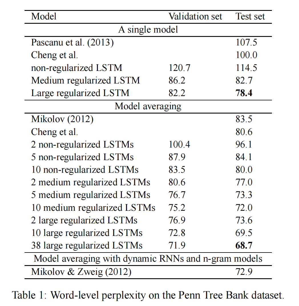

The medium LSTM has 650 units per layer and its parameters are initialized uniformly in [−0.05, 0.05]. As described earlier, we apply 50% dropout on the non-recurrent connections. We train the LSTM for 39 epochs with a learning rate of 1, and after 6 epochs we decrease it by a factor of 1.2 after each epoch. We clip the norm of the gradients (normalized by minibatch size) at 5. Training this network takes about half a day on an NVIDIA K20 GPU.
中型LSTM每层有650个单元，其参数在[−0.05, 0.05]范围内均匀初始化。如前所述，我们在非递归连接上应用50%的dropout。我们用学习率为1训练LSTM共39个周期，在第6个周期后，每个周期将学习率按1.2的因子递减。我们将梯度的范数（按小批量大小归一化）剪裁到5。训练该网络在NVIDIA K20 GPU上大约需要半天时间。

The large LSTM has 1500 units per layer and its parameters are initialized uniformly in [−0.04, 0.04]. We apply 65% dropout on the non-recurrent connections. We train the model for 55 epochs with a learning rate of 1; after 14 epochs we start to reduce the learning rate by a factor of 1.15 after each epoch. We clip the norm of the gradients (normalized by minibatch size) at 10 Mikolov et al. (2010). Training this network takes an entire day on an NVIDIA K20 GPU.
大型LSTM每层有1500个单元，其参数在[−0.04, 0.04]范围内均匀初始化。我们在非递归连接上应用65%的dropout。我们用学习率为1训练模型共55个周期；在第14个周期后，每个周期开始按1.15的因子递减学习率。我们将梯度的范数（按小批量大小归一化）剪裁到10 Mikolov等（2010）。训练该网络在NVIDIA K20 GPU上需要整整一天时间。

For comparison, we trained a non-regularized network. We optimized its parameters to get the best validation performance. The lack of regularization effectively constrains size of the network, forcing us to use small network because larger networks overfit. Our best performing non-regularized LSTM has two hidden layers with 200 units per layer, and its weights are initialized uniformly in [−0.1, 0.1]. We train it for 4 epochs with a learning rate of 1 and then we decrease the learning rate by a factor of 2 after each epoch, for a total of 13 training epochs. The size of each minibatch is 20, and we unroll the network for 20 steps. Training this network takes 2-3 hours on an NVIDIA K20 GPU.
为了比较，我们训练了一个未正则化的网络。我们优化其参数以获得最佳验证性能。缺乏正则化有效地限制了网络的大小，迫使我们使用小型网络，因为较大的网络会过拟合。我们表现最好的未正则化LSTM有两层隐藏层，每层200个单元，其权重在[−0.1, 0.1]范围内均匀初始化。我们用学习率为1训练了4个周期，然后每个周期将学习率按2的因子递减，总共训练13个周期。每个小批量的大小为20，我们展开网络20步。训练该网络在NVIDIA K20 GPU上需要2-3小时。

Table 1 compares previous results with our LSTMs, and Figure 4 shows samples drawn from a single large regularized LSTM.
表1比较了以前的结果和我们的LSTM，图4显示了从单个大型正则化LSTM中抽取的样本。

4.2 SPEECH RECOGNITION 语音识别

Deep Neural Networks have been used for acoustic modeling for over half a century (see Bourlard & Morgan (1993) for a good review). Acoustic modeling is a key component in mapping acoustic signals to sequences of words, as it models $p(s_t|X)$ where $s_t$​ is the phonetic state at time $t$ and $X$ is the acoustic observation. Recent work has shown that LSTMs can achieve excellent performance on acoustic modeling Sak et al. (2014), yet relatively small LSTMs (in terms of the number of their parameters) can easily overfit the training set. A useful metric for measuring the performance of acoustic models is frame accuracy, which is measured at each sts_tst​ for all timesteps ttt. Generally, this metric correlates with the actual metric of interest, the Word Error Rate (WER).
深度神经网络已经被用于声学建模超过半个世纪（参见Bourlard & Morgan (1993)的良好综述）。声学建模是将声学信号映射到单词序列中的关键组成部分，因为它对p(st∣X)p(s_t|X)p(st​∣X)建模，其中sts_tst​是时间ttt的语音状态，XXX是声学观测。最近的工作表明，LSTM在声学建模上可以取得优异的性能 Sak等（2014），但相对较小的LSTM（就参数数量而言）很容易对训练集过拟合。衡量声学模型性能的一个有用指标是帧准确率，它在所有时间步长ttt处测量每个sts_tst​的准确率。通常，这个指标与实际感兴趣的指标，即单词错误率（WER）相关。

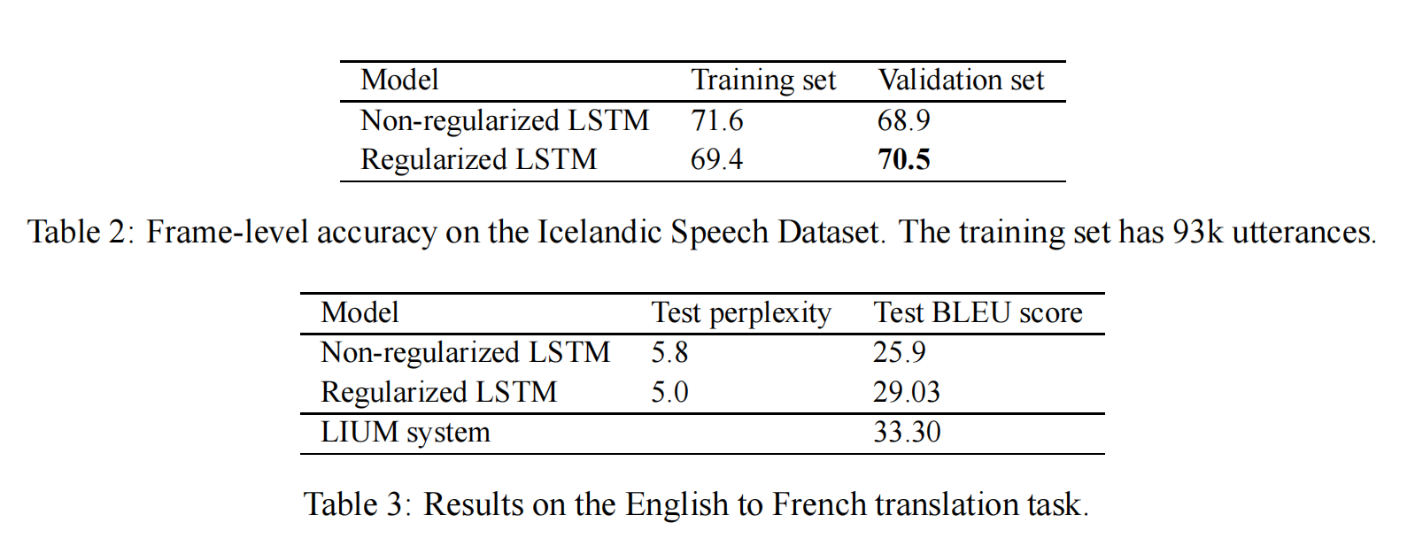
Since computing the WER involves using a language model and tuning the decoding parameters for every change in the acoustic model, we decided to focus on frame accuracy in these experiments. Table 2 shows that dropout improves the frame accuracy of the LSTM. Not surprisingly, the training frame accuracy drops due to the noise added during training, but as is often the case with dropout, this yields models that generalize better to unseen data. Note that the test set is easier than the training set, as its accuracy is higher. We report the performance of an LSTM on an internal Google Icelandic Speech dataset, which is relatively small (93k utterances), so overfitting is a great concern.
由于计算WER涉及使用语言模型并调整声学模型每次变化的解码参数，我们决定在这些实验中专注于帧准确率。表2显示了dropout提高了LSTM的帧准确率。不出所料，由于训练过程中加入的噪声，训练帧准确率下降了，但与dropout经常出现的情况一样，这使得模型在未见数据上的泛化能力更强。请注意，测试集比训练集更容易，因为它的准确率更高。我们报告了LSTM在Google内部冰岛语语音数据集上的性能，该数据集相对较小（93k句子），因此过拟合是一个很大的问题。

4.3 MACHINE TRANSLATION 机器翻译

We formulate a machine translation problem as a language modelling task, where an LSTM is trained to assign high probability to a correct translation of a source sentence. Thus, the LSTM is trained on concatenations of source sentences and their translations Sutskever et al. (2014) (see also Cho et al. (2014)). We compute a translation by approximating the most probable sequence of words using a simple beam search with a beam of size 12. We ran an LSTM on the WMT’14 English to French dataset, on the “selected” subset from Schwenk (2014) which has 340M French words and 304M English words. Our LSTM has 4 hidden layers, and both its layers and word embeddings have 1000 units. Its English vocabulary has 160,000 words and its French vocabulary has 80,000 words. The optimal dropout probability was 0.2. Table 3 shows the performance of an LSTM trained with and without dropout. While our LSTM does not beat the phrase-based LIUM SMT system Schwenk et al. (2011), our results show that dropout improves the translation performance of the LSTM.
我们将机器翻译问题表述为一个语言建模任务，其中LSTM被训练为对源句子的正确翻译赋予高概率。因此，LSTM在源句子及其翻译的串联上进行训练 Sutskever等（2014）（另见Cho等（2014））。我们通过使用大小为12的简单束搜索来近似最可能的单词序列来计算翻译。我们在WMT’14英法数据集上的“selected”子集（来自Schwenk（2014），包含3.4亿个法语单词和3.04亿个英语单词）上运行了一个LSTM。我们的LSTM有4个隐藏层，其层和词嵌入都有1000个单元。它的英语词汇量有160,000个单词，法语词汇量有80,000个单词。最佳的dropout概率是0.2。表3显示了使用和不使用dropout训练的LSTM的性能。虽然我们的LSTM没有击败基于短语的LIUM SMT系统 Schwenk等（2011），但我们的结果表明dropout提高了LSTM的翻译性能。

4.4 IMAGE CAPTION GENERATION图像描述生成

We applied the dropout variant to the image caption generation model of Vinyals et al. (2014). The image caption generation is similar to the sequence-to-sequence model of Sutskever et al. (2014), but where the input image is mapped onto a vector with a highly-accurate pre-trained convolutional neural network (Szegedy et al., 2014), which is converted into a caption with a single-layer LSTM (see Vinyals et al. (2014) for the details on the architecture). We test our dropout scheme on LSTM as the convolutional neural network is not trained on the image caption dataset because it is not large (MSCOCO (Lin et al., 2014)).
我们将dropout变体应用于Vinyals等人（2014）的图像描述生成模型。图像描述生成类似于Sutskever等人（2014）的序列到序列模型，但输入图像被映射到一个具有高精度的预训练卷积神经网络（Szegedy等人，2014）的向量，该向量通过单层LSTM转换为描述（有关架构的详细信息，请参见Vinyals等人，2014）。我们在LSTM上测试了我们的dropout方案，因为卷积神经网络并未在图像描述数据集上进行训练，因为它不是很大（MSCOCO（Lin等人，2014））。

Our results are summarized in the following Table 4. In brief, dropout helps relative to not using dropout, but using an ensemble eliminates the gains attained by dropout. Thus, in this setting, the main effect of dropout is to produce a single model that is as good as an ensemble, which is a reasonable improvement given the simplicity of the technique.
我们的结果总结在以下表4中。简而言之，dropout相对于不使用dropout有帮助，但使用集成方法消除了通过dropout获得的收益。因此，在这种情况下，dropout的主要作用是产生一个与集成一样好的单一模型，考虑到该技术的简单性，这是一个合理的改进。

5 CONCLUSION

We presented a simple way of applying dropout to LSTMs that results in large performance increases on several problems in different domains. Our work makes dropout useful for RNNs, and our results suggest that our implementation of dropout could improve performance on a wide variety of applications.
我们提出了一种将dropout应用于LSTM的简单方法，这在不同领域的几个问题上导致了性能的大幅提升。我们的工作使dropout对RNN有用，并且我们的结果表明，我们实现的dropout可以提高各种应用的性能。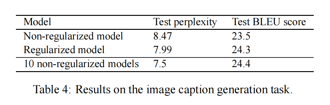

6 ACKNOWLEDGMENTS

We wish to acknowledge Tomas Mikolov for useful comments on the first version of the paper.
我们希望感谢Tomas Mikolov对论文第一版提出的有益意见。

注释

1. 元素乘法

元素乘法（Element-wise multiplication），也称为Hadamard乘积（Hadamard product），是对两个同形矩阵或向量的对应元素进行逐一相乘的操作，广泛应用于各种线性代数和神经网络计算中。 用符号“⊙”表示。

公式表示

给定两个相同大小的矩阵或向量 $A$ 和 $B$，其元素乘法 $C$ 计算如下：
$C = A \odot B$

其中：

• $A = [a_1, a_2, …, a_n]$
• $B = [b_1, b_2, …, b_n]$
• $C = [c_1, c_2, …, c_n]$
• $c_i = a_i \cdot b_i$

  示例

假设有两个向量 $A$ 和 $B$：

$A=[1,2,3]$
$B=[4,5,6]$

它们的元素乘法 $C$ 为：
$C = A \odot B = [1 \cdot 4, 2 \cdot 5, 3 \cdot 6] = [4, 10, 18]$

应用场景

1. 神经网络中的LSTM：
   • 用于更新单元状态，如公式 $c_t = f \odot c_{t-1} + i \odot \tilde{c}_t$中。
2. 图像处理：
   • 用于图像滤波，将滤波器应用于图像的每个像素。
3. 数据处理：
   • 在数据预处理中，用于按元素缩放或调整数据。

2. 公式拆解:RNN

RNN : $h_t^{l-1}​$, $h_{t-1}^l \rightarrow h_t^l$

表明在RNN中， 隐藏状态的计算结果依赖于当前时间步的输入 $h_t$和前一时间步的隐藏状态 $h_{t-1}$。 再细化一点，

1. 当前时间步的输入 $h_t$ 应该来源于上一层，所以是 $h_t^{l-1}​$
2. 前一时间步的隐藏状态 $h_{t-1}$ ，应该是同一层的前一个时间步， 所以是$h_{t-1}^l$

该状态转移过程，如果用具体的数学公式表示，可以如下所示
$h_t^l = f(T_{n,n} h_t^{l-1} + T_{n,n} h_{t-1}^l), where f \in \{\text{sigm, tanh}\}$

3. 公式拆解:LSTM 状态更新

LSTM : $h_t^{l-1}$, $h_{t-1}^l$, $c_{t-1}^l \rightarrow h_t^l$​, $c_t^l$
描述了LSTM如何通过当前层的输入向量 $h_t^{l-1}$、前一时间步的隐藏状态 $h_{t-1}^l$和单元状态 $c_{t-1}^l$ 来生成新的隐藏状态 $h_t^l$ 和单元状态 $c_t^l$。

1. $h_t^{l-1}$：表示第 $l−1$ 层在时间步 $t$ 的隐藏状态向量。这是第 $l$ 层的当前输入。
2. $h_{t-1}^l$：表示第 $l$ 层在时间步 $t−1$ 的隐藏状态向量。这是第 $l$ 层的前一个时间步的状态。
3. $c_{t-1}^l$：表示第 $l$ 层在时间步 $t−1$的单元状态向量。这是第 $l$ 层的前一个时间步的单元状态。
4. $h_t^l$：表示第 $l$ 层在时间步 $t$ 的隐藏状态向量。这是经过第 $l$ 层计算后的新状态。
5. $c_t^l$：表示第 $l$ 层在时间步 $t$ 的新的单元状态向量。这是更新后的单元状态。

$\left( \begin{array}{c} i \ f \ o \ g \end{array} \right) = \left( \begin{array}{c} \text{sigm} \ \text{sigm} \ \text{sigm} \ \text{tanh} \end{array} \right) T_{2n,4n} \left( \begin{array}{c} h_{t}^{l-1} \ h_{t-1}^{l} \end{array} \right)​$

描述了输入门 $i$、遗忘门 $f$、输出门 $o$ 和候选记忆单元 $g$ 的计算。这里，矩阵 $T_{2n,4n}$​ 包含了相应的权重，输入包括当前输入 $h_t^{l-1}$和前一时间步的隐藏状态 $h_{t-1}^l$​

• 输入门 $i$ 和 遗忘门 $f$ 控制信息的更新和遗忘，使用$sigmoid$激活函数。
• 输出门 $o$ 控制输出信息，使用$sigmoid$激活函数。
• 候选记忆单元 $g$ 提供新的信息内容，使用$tanh$激活函数。
• 权重矩阵 $T_{2n,4n}$ 一个大小为 $2n \times 4n$ 的矩阵，其中 $n$ 是隐藏状态向量的维度。将输入向量 $h_t^{l-1}$​ 和隐藏状态向量 $h_{t-1}^l$ 拼接起来（向量长度为 $2n$），并通过矩阵 $T_{2n,4n}$​ 进行线性变换，生成一个长度为 $4n$ 的输出向量,即 $i, f, o, g$ 四个部分

  1. 遗忘门（Forget Gate）

$f_t^l = \sigma(W_f \cdot [h_{t-1}^l, h_t^{l-1}] + b_f)$

• $[h_t^{l-1}, h_{t-1}^l]$表示将当前输入和前一时间步的隐藏状态向量拼接成一个向量。
• $W_f​$ 是该拼接向量的权重矩阵。
• $b_f$​ 是偏置向量。
• $\sigma$ 是$sigmoid$激活函数，输出范围在0到1之间。

假设 $n = 4$：

• 当前输入向量 $h_t^{l-1}$为 $[h_1​,h_2​,h_3​,h_4​]$。
• 前一时间步的隐藏状态 $h_{t-1}^l$ 为 $[h_5, h_6, h_7, h_8]$

拼接后的向量为：$[h_1, h_2, h_3, h_4, h_5, h_6, h_7, h_8]$

权重矩阵 $W_f​$ 将此向量进行线性变换，生成一个长度为 $n$ 的向量。

线性变换

进行线性变换的公式为：
$z_f = W_f \cdot [h_t^{l-1}, h_{t-1}^l] + b_f$

具体步骤：

1. 矩阵乘法：
   • $W_f$是一个 $n \times 2n$ 的矩阵，拼接向量是一个长度为 $2n$ 的向量。
   • 通过矩阵乘法，结果是一个长度为 $n$ 的向量。
2. 加偏置：
   • 将得到的向量与偏置向量 $b_f$ 相加，仍然是一个长度为 $n$ 的向量。

例如，假设 $W_f$​ 和 $b_f$​ 为：
$W_f = \begin{pmatrix} w_{11} & w_{12} & w_{13} & w_{14} & w_{15} & w_{16} & w_{17} & w_{18} \ w_{21} & w_{22} & w_{23} & w_{24} & w_{25} & w_{26} & w_{27} & w_{28} \ w_{31} & w_{32} & w_{33} & w_{34} & w_{35} & w_{36} & w_{37} & w_{38} \ w_{41} & w_{42} & w_{43} & w_{44} & w_{45} & w_{46} & w_{47} & w_{48} \end{pmatrix}$

拼接向量为：
$[h_1, h_2, h_3, h_4, h_5, h_6, h_7, h_8]$

矩阵乘法：
$z_f = W_f \cdot [h_1, h_2, h_3, h_4, h_5, h_6, h_7, h_8]$

计算每个元素：
$\begin{aligned} z_{f1} &= w_{11}h_1 + w_{12}h_2 + w_{13}h_3 + w_{14}h_4 + w_{15}h_5 + w_{16}h_6 + w_{17}h_7 + w_{18}h_8 \ z_{f2} &= w_{21}h_1 + w_{22}h_2 + w_{23}h_3 + w_{24}h_4 + w_{25}h_5 + w_{26}h_6 + w_{27}h_7 + w_{28}h_8 \ z_{f3} &= w_{31}h_1 + w_{32}h_2 + w_{33}h_3 + w_{34}h_4 + w_{35}h_5 + w_{36}h_6 + w_{37}h_7 + w_{38}h_8 \ z_{f4} &= w_{41}h_1 + w_{42}h_2 + w_{43}h_3 + w_{44}h_4 + w_{45}h_5 + w_{46}h_6 + w_{47}h_7 + w_{48}h_8 \end{aligned}$

加偏置：
$z_f = \begin{pmatrix} z_{f1} + b_1 \ z_{f2} + b_2 \ z_{f3} + b_3 \ z_{f4} + b_4 \end{pmatrix}$

sigmoid 非线性激活

通过$sigmoid$激活函数得到遗忘门的激活值：
$f_t^l = \sigma(z_f)$
通过 $sigmoid$ 非线性激活函数，得到遗忘门的激活值。

2. 输入门（Input Gate）

计算输入门的激活值，决定新的输入信息的哪些部分将更新单元状态： $i_t^l = \sigma(W_i \cdot [h_{t-1}^l, h_t^{l-1}] + b_i)$

输入调制门（Input Modulation Gate）输入调制门产生新的候选记忆内容，通过 tanh 函数进行激活。
它的数学表示为：$g_t = \tanh(W_g \cdot [h_{t-1}, h_t] + b_g)$

3. 单元状态

结合遗忘门和输入门的信息，更新单元状态：

$c_t^l = f \odot c_{t-1}^l + i \odot g$

描述了如何更新单元状态。这里，$\odot$ 表示元素乘法（Hadamard乘积）。

• 遗忘门$f$决定了前一时间步的单元状态 $c_{t-1}^l$有多少被保留。遗忘门的输出值在0和1之间：
  • 当 $f$​ 接近1时，表示大部分单元状态被保留。
  • 当 $f$接近0时，表示大部分单元状态被遗忘。
• 输入门 $i$ 和候选记忆单元 $g$ 决定了多少新的信息被添加到当前单元状态 $c_t^l$。

4. 输出门

计算输出门的激活值，决定隐藏状态的更新：
输出门：$o_t^l = \sigma(W_o \cdot [h_{t-1}^l, h_t^{l-1}] + b_o)$
隐藏状态：$h_t^l = o_t^l * \tanh(c_t^l)$
输出门 $o$ 控制了从单元状态 $c_t^l$ 传递到隐藏状态 $h_t^l$​ 的信息，通过$tanh$函数进行非线性变换。

LSTM通过输入门、遗忘门、输出门和候选记忆单元的协同作用，有效地捕捉序列数据中的长短期依赖关系，解决了传统RNN中梯度消失和梯度爆炸的问题。这个更新机制使得LSTM在处理长序列数据时表现出色，能够有效地保留重要信息并过滤无关信息。

5. 更新隐藏状态（Hidden State Update）

结合新的单元状态和输出门的激活值，更新隐藏状态： $h_t^l = o_t^l * \tanh(c_t^l)$

4. 应用了dropout 的LSTM

从正文中可以看出，和标准的LSTM 状态更新过程相比， 其变化只是增加了一个$D$。
$D$ 是将其参数的随机子集设置为零的dropout操作符。

$\left( \begin{array}{c} i \ f \ o \ g \end{array} \right) = \left( \begin{array}{c} \text{sigm} \ \text{sigm} \ \text{sigm} \ \text{tanh} \end{array} \right) T_{2n,4n} \left( \begin{array}{c} {D}(h_{t}^{l-1}) \ h_{t-1}^{l} \end{array} \right)​$

如何理解其主要思想是仅将dropout操作符应用于非递归连接。
由于：

1. $h_t^{l-1}$：表示第 $l−1$ 层在时间步 $t$ 的隐藏状态向量。这是第 $l$ 层的当前输入。
2. $h_{t-1}^l$：表示第 $l$ 层在时间步 $t−1$ 的隐藏状态向量。这是第 $l$ 层的前一个时间步的状态。
   同一层前后时间步之间的数据流转 就是递归操作， 不同层之间的数据流转是非递归操作， 根据公式，$D$ 应用在了$h_t^{l-1}$上， 所以说$D$ 是应用在非递归连接上的操作符合